14.1. Definition of Attention Mechanism
Attention mechanisms come in many variations and extensions, as summarized in the following papers:
Here, we will focus on the two novel attention mechanisms proposed in the first two papers: the Bahdanau and Luong styles, which share similar structures with other variations.
14.1.1. Definition
The attention mechanism can be mathematically expressed as follows:
$$ \text{Attention}(q_{i}) = \sum^{n}_{j=1} \text{softmax}(\text{score}(q_{i}, k_{j})) v_{j} = \sum^{n}_{j=1} a(q_{i}, k_{j}) v_{j} \tag{14.1} $$where:
- $q \in \mathbb{R}^{d_{q}} $ is a query vector, $Q = [ q_{1}, q_{2},\ldots, q_{m} ] \in \mathbb{R}^{d_{q} \times m } $ is a set of query vectors.
- $k \in \mathbb{R}^{d_{k}} $ is a key vector, $K = [ k_{1}, k_{2},\ldots, k_{n} ] \in \mathbb{R}^{d_{k} \times n } $ is a set of key vectors.
- $v \in \mathbb{R}^{d_{v}} $ is a value vector, $V = [ v_{1}, v_{2},\ldots, v_{n} ] \in \mathbb{R}^{d_{v} \times n } $ is a set of value vectors.
- $\text{score}(q_{i}, k_{j})$ is a function that computes the similarity between a query $q_{i}$ and a key $k_{j}$.
- $a(q_{i}, k_{j}) \stackrel{\mathrm{def}}{=} \text{softmax}(\text{score}(q_{i}, k_{j})) $ is an attention weight.
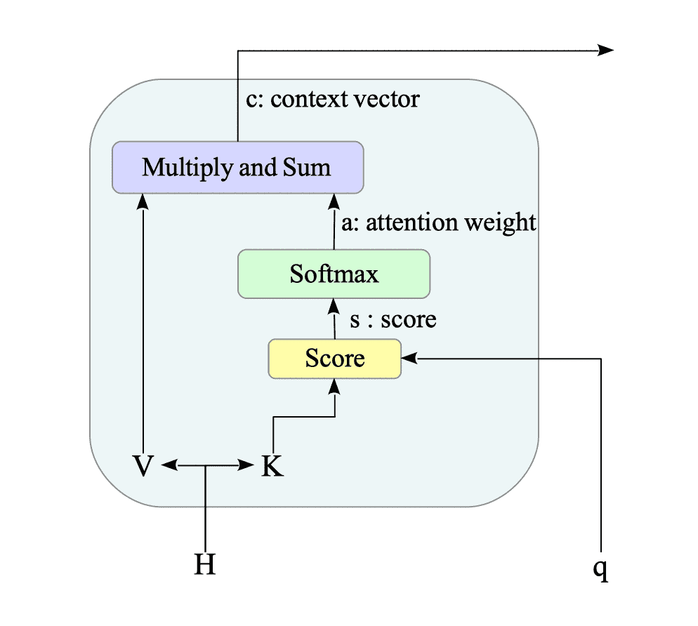
Fig.14-2 illustrates a typical attention model architecture:

Fig.14-2: Attention Model Architecture
Here is a breakdown of how it works:
As shown in Fig.14-2, $K$ and $V$ are usually the same matrix, represented as $ H = [ h_{1}, h_{2},\ldots, h_{n} ] \in \mathbb{R}^{ d_{h} \times n } $. In RNN based encoder-decoder models, $H$ is the hidden states of the encoder.
Some major score functions, which compute the similarity between a query $q_{i}$ and a key $k_{j}$, are shown as follows:
$$ \begin{align} \text{score}(q_{i}, k_{j}) = & \begin{cases} q^{T}_{i} W_{\alpha} k_{j} & \text{[General]} \\ V_{\alpha}^{T} \tanh(W_{\alpha} [q_{i}; k_{j}]) & \text{[Concat]} \\ V_{\alpha}^{T} \tanh(W_{1} q_{i} + W_{2} k_{j} + b) & \text{[Additive]} \\ q^{T}_{i} k_{j} & \text{[Dot-Product]} \end{cases} \end{align} \tag{14.2} $$where $W_{\alpha}, W_{1}, W_{2}$ and $V_{\alpha}$ are weight matrices, and $b$ is a bias. They are learnable, i.e., they will be set to appropriate values by training.
This score is then normalized using the softmax function to obtain the attention weight:
$$ a(q_{i}, k_{j}) \stackrel{\mathrm{def}}{=} \text{softmax}(\text{score}(q_{i}, k_{j})) $$It satisfies $ a(q_{i}, k_{j}) \in [0,1] $ and $\sum_{j} a(q_{i}, k_{j}) = 1$.
The attention weight reflects the importance of key $k_{j}$ for query $q_{i}$ in the current context.
The attention weights are multiplied by the corresponding encoder output vectors $v_{j} \in \mathbb{R}^{d_{v}}$, effectively emphasizing relevant information:
$$ a(q_{i}, k_{j}) v_{j} $$The weighted vectors $a(q_{i}, k_{j}) v_{j}$ are then summed to create the attention output, which represents a condensed representation of the encoder sequence focused on the decoder’s current needs.
$$ \sum_{j} a(q_{i}, k_{j}) v_{j} $$The output of the attention mechanism is often referred to as the context vector. For example, in machine translation, these attention outputs are used as context vectors for the decoder.
14.1.2. Intuitive explanation of score functions
Consider measuring the similarity between two word pairs with equivalent meanings in Spanish and English:
- “Sol” and “Sun” ☀️
- “Lluvia” and “Rain” ☔
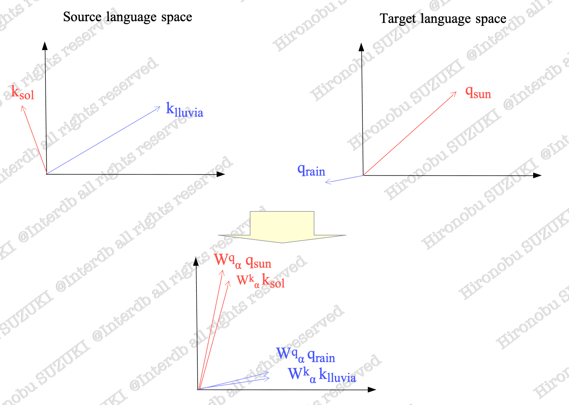
These words are embedded in their respective language spaces as vectors ($k_{\text{sol}}$ and $k_{\text{llvia}}$ in Spanish, $q_{\text{sun}}$ and $q_{\text{rain}}$ in English) using distinct embedding methods.
Although these words have the same meaning in both languages, the vectors $k_{\text{sol}}$ and $q_{\text{sun}}$ may not be similar in the embedding space because different languages use different embedding methods.

Fig.14-3: (Top) Word Vectors in Each Language Space. (Bottom) Word Vectors Multiplied by Matrices.
To measure similarity between vectors from different spaces, we introduce transforming them with matrix.
By choosing appropriate matrices $W_{\alpha}^{q}$ and $W_{\alpha}^{k}$ such that $(W_{\alpha}^{q})^T W_{\alpha}^{k} = W_{\alpha}$, we can make the vectors $W_{\alpha}^{q} q_{\text{sun}}$ and $W_{\alpha}^{k} k_{\text{sol}}$ more similar. The same applies to the other pair, $W_{\alpha}^{q} q_{\text{rain}}$ and $W_{\alpha}^{k} k_{\text{lluvia}}$.
Now, let’s compute the similarity between $W_{\alpha}^{q} q_{\text{sun}}$ and $W_{\alpha}^{k} k_{\text{sol}}$ using the dot product:
$$ (W_{\alpha}^{q} q_{\text{sun}})^{T} W_{\alpha}^{k} k_{\text{sol}} = q_{\text{sun}}^{T} (W_{\alpha}^{q})^{T} W_{\alpha}^{k} k_{\text{sol}} = q_{\text{sun}}^{T} W_{\alpha} k_{\text{sol}} \tag{14.3} $$This dot product $(14.3)$ is the general score function in $(14.2)$ itself.
Clearly, matrix $W_{\alpha}$ plays a crucial role in connecting the two language spaces1. We can obtain an appropriate matrix through training.
In general, score functions require learnable parameters. The learnability of the score functions makes it possible to compute the similarity between $q$ and $k$ vectors, each belonging to a different language space2.
-
For simplicity, this explanation uses learning relationships between words as an example. However, as we will show in the following sections, we deal with sentences as inputs, which are sequences of words. Therefore, the weight matrix $ W_{\alpha} $ learns the relationship between words in two language spaces considering the context of the sentences, including the order and surrounding words. ↩︎
-
If $q$ and $k$ have already been vectorized considering their similarity, you can use the Dot-Product score function: $q^{T} k$ ↩︎