3.2. Cost Estimation in Single-Table Query
PostgreSQL’s query optimization is based on cost. Costs are dimensionless values, and they are not absolute performance indicators, but rather indicators to compare the relative performance of operations.
Costs are estimated by the functions defined in costsize.c. All operations executed by the executor have corresponding cost functions. For example, the costs of sequential scans and index scans are estimated by cost_seqscan() and cost_index(), respectively.
In PostgreSQL, there are three kinds of costs: start-up, run and total. The total cost is the sum of the start-up and run costs, so only the start-up and run costs are independently estimated.
- The start-up cost is the cost expended before the first tuple is fetched. For example, the start-up cost of the index scan node is the cost of reading index pages to access the first tuple in the target table.
- The run cost is the cost of fetching all tuples.
- The total cost is the sum of the costs of both start-up and run costs.
The EXPLAIN command shows both of start-up and total costs in each operation. The simplest example is shown below:
|
|
In Line 4, the command shows information about the sequential scan. In the cost section, there are two values; 0.00 and 145.00. In this case, the start-up and total costs are 0.00 and 145.00, respectively.
In this section, we will explore how to estimate the sequential scan, index scan, and sort operation in detail.
In the following explanations, we will use a specific table and an index that are shown below:
testdb=# CREATE TABLE tbl (id int PRIMARY KEY, data int);
testdb=# CREATE INDEX tbl_data_idx ON tbl (data);
testdb=# INSERT INTO tbl SELECT generate_series(1,10000),generate_series(1,10000);
testdb=# ANALYZE;
testdb=# \d tbl
      Table "public.tbl"
 Column |  Type   | Modifiers
--------+---------+-----------
 id     | integer | not null
 data   | integer |
Indexes:
    "tbl_pkey" PRIMARY KEY, btree (id)
"tbl_data_idx" btree (data)3.2.1. Sequential Scan
The cost of the sequential scan is estimated by the cost_seqscan() function. In this subsection, we will explore how to estimate the sequential scan cost of the following query:
testdb=# SELECT * FROM tbl WHERE id <= 8000;In the sequential scan, the start-up cost is equal to 0, and the run cost is defined by the following equation:
$$ \begin{align} \text{'run cost'} &= \text{'cpu run cost'} + \text{'disk run cost'} \\ &= (\text{cpu_tuple_cost} + \text{cpu_operator_cost}) \times N_{tuple} + \text{seq_page_cost} \times N_{page} \end{align} $$where seq_page_cost, cpu_tuple_cost and cpu_operator_cost are set in the postgresql.conf file, and the default values are 1.0, 0.01, and 0.0025, respectively. $ N_{tuple} $ and $ N_{page} $ are the numbers of all tuples and all pages of this table, respectively. These numbers can be shown using the following query:
testdb=# SELECT relpages, reltuples FROM pg_class WHERE relname = 'tbl';
 relpages | reltuples
----------+-----------
       45 |     10000
(1 row)Therefore,
$$ \begin{align} \text{'run cost'} &= (0.01 + 0.0025) \times 10000 + 1.0 \times 45 = 170.0 \end{align} $$Finally,
$$ \begin{align} \text{'total cost'} = 0.0 + 170.0 = 170 \end{align} $$For confirmation, the result of the EXPLAIN command of the above query is shown below:
|
|
In Line 4, we can see that the start-up and total costs are 0.00 and 170.00, respectively. It is also estimated that 8000 rows (tuples) will be selected by scanning all rows.
In line 5, a filter ‘$\text{Filter}:(\text{id} \lt= 8000)$’ of the sequential scan is shown. More precisely, it is called a table level filter predicate.
Note that this type of filter is used when reading all the tuples in the table, and it does not narrow the scanned range of table pages.
As understood from the run-cost estimation, PostgreSQL assumes that all pages will be read from storage. In other words, PostgreSQL does not consider whether the scanned page is in the shared buffers or not.
3.2.2. Index Scan
Although PostgreSQL supports some index methods, such as BTree, GiST, GIN and BRIN, the cost of the index scan is estimated using the common cost function cost_index().
In this subsection, we explore how to estimate the index scan cost of the following query:
testdb=# SELECT id, data FROM tbl WHERE data <= 240;Before estimating the cost, the numbers of the index pages and index tuples, $ N_{index,page} $ and $ N_{index,tuple} $, are shown below:
testdb=# SELECT relpages, reltuples FROM pg_class WHERE relname = 'tbl_data_idx';
 relpages | reltuples
----------+-----------
       30 |     10000
(1 row)3.2.2.1. Start-Up Cost
The start-up cost of the index scan is the cost of reading the index pages to access the first tuple in the target table. It is defined by the following equation:
$$ \begin{align} \text{'start-up cost'} = \{\mathrm{ceil}(\log_2 (N_{index,tuple})) + (H_{index} + 1) \times 50\} \times \text{cpu_operator_cost} \end{align} $$where $ H_{index} $ is the height of the index tree. The detail of this calculation is explained in the comments of btcostestimate().
In this case, according to (3), $ N_{index,tuple} $ is 10000, $ H_{index} $ is 1; $ \text{cpu_operator_cost} $ is $0.0025$ (by default). Therefore,
$$ \begin{align} \text{'start-up cost'} = \{\mathrm{ceil}(\log_2(10000)) + (1 + 1) \times 50\} \times 0.0025 = 0.285 \tag{5} \end{align} $$3.2.2.2. Run Cost
The run cost of the index scan is the sum of the CPU costs and the I/O (input/output) costs of both the table and the index:
$$ \begin{align} \text{'run cost'} &= (\text{'index cpu cost'} + \text{'table cpu cost'}) + (\text{'index IO cost'} + \text{'table IO cost'}). \end{align} $$If the Index-Only Scans, which is described in Section 7.2, can be applied, $ \text{’table cpu cost’} $ and $ \text{’table IO cost’} $ are not estimated.
The first three costs (i.e., index CPU cost, table CPU cost, and index I/O cost) are shown below:
$$ \begin{align} \text{'index cpu cost'} &= \text{Selectivity} \times N_{index,tuple} \times (\text{cpu_index_tuple_cost} + \text{qual_op_cost}) \\ \text{'table cpu cost'} &= \text{Selectivity} \times N_{tuple} \times \text{cpu_tuple_cost} \\ \text{'index IO cost'} &= \mathrm{ceil}(\text{Selectivity} \times N_{index,page}) \times \text{random_page_cost} \end{align} $$where:
- cpu_index_tuple_cost and random_page_cost are set in the postgresql.conf file. The defaults are 0.005 and 4.0, respectively.
- $ \text{qual_op_cost} $ is, roughly speaking, the cost of evaluating the index predicate. The default is 0.0025.
- $ \text{Selectivity} $ is the proportion of the search range of the index that satisfies the WHERE clause, it is a floating-point number from 0 to 1.
$ (\text{Selectivity} \times N_{tuple}) $ means the number of the table tuples to be read;
$ (\text{Selectivity} \times N_{index,page}) $ means the number of the index pages to be read.
Selectivity is described in detail in below.
The selectivity of query predicates is estimated using either the histogram_bounds or the MCV (Most Common Value), both of which are stored in the statistics information in the pg_stats.
Here, the calculation of the selectivity is briefly described using specific examples.
More details are provided in the official document.
The MCV of each column of a table is stored in the pg_stats view as a pair of columns named ‘most_common_vals’ and ‘most_common_freqs’:
- ‘most_common_vals’ is a list of the MCVs in the column.
- ‘most_common_freqs’ is a list of the frequencies of the MCVs.
Here is a simple example:
The table “countries” has two columns:
- a column ‘country’: This column stores the country name.
- a column ‘continent’: This column stores the continent name to which the country belongs.
testdb=# \d countries
   Table "public.countries"
  Column   | Type | Modifiers
-----------+------+-----------
 country   | text |
 continent | text |
Indexes:
    "continent_idx" btree (continent)

testdb=# SELECT continent, count(*) AS "number of countries",
testdb-#     (count(*)/(SELECT count(*) FROM countries)::real) AS "number of countries / all countries"
testdb-#       FROM countries GROUP BY continent ORDER BY "number of countries" DESC;
   continent   | number of countries | number of countries / all countries
---------------+---------------------+-------------------------------------
 Africa        |                  53 |                   0.274611398963731
 Europe        |                  47 |                   0.243523316062176
 Asia          |                  44 |                   0.227979274611399
 North America |                  23 |                   0.119170984455959
 Oceania       |                  14 |                  0.0725388601036269
 South America |                  12 |                  0.0621761658031088
(6 rows)
Consider the following query, which has a WHERE clause, ‘continent = ‘Asia’’:
testdb=# SELECT * FROM countries WHERE continent = 'Asia';In this case, the planner estimates the index scan cost using the MCV of the ‘continent’ column. The ‘most_common_vals’ and ‘most_common_freqs’ of this column are shown below:
testdb=# \x
Expanded display is on.
testdb=# SELECT most_common_vals, most_common_freqs FROM pg_stats
testdb-#                  WHERE tablename = 'countries' AND attname='continent';
-[ RECORD 1 ]-----+-------------------------------------------------------------
most_common_vals  | {Africa,Europe,Asia,"North America",Oceania,"South America"}
most_common_freqs | {0.274611,0.243523,0.227979,0.119171,0.0725389,0.0621762}
The value of most_common_freqs corresponding to ‘Asia’ of the most_common_vals is 0.227979. Therefore, 0.227979 is used as the selectivity in this estimation.
If the MCV cannot be used, e.g., the target column type is integer or double precision, then the value of the histogram_bounds of the target column is used to estimate the cost.
- histogram_bounds is a list of values that divide the column’s values into groups of approximately equal population.
A specific example is shown. This is the value of the histogram_bounds of the column ‘data’ in the table ’tbl’:
testdb=# SELECT histogram_bounds FROM pg_stats WHERE tablename = 'tbl' AND attname = 'data';
        			     	      histogram_bounds
---------------------------------------------------------------------------------------------------
 {1,100,200,300,400,500,600,700,800,900,1000,1100,1200,1300,1400,1500,1600,1700,1800,1900,2000,2100,
2200,2300,2400,2500,2600,2700,2800,2900,3000,3100,3200,3300,3400,3500,3600,3700,3800,3900,4000,4100,
4200,4300,4400,4500,4600,4700,4800,4900,5000,5100,5200,5300,5400,5500,5600,5700,5800,5900,6000,6100,
6200,6300,6400,6500,6600,6700,6800,6900,7000,7100,7200,7300,7400,7500,7600,7700,7800,7900,8000,8100,
8200,8300,8400,8500,8600,8700,8800,8900,9000,9100,9200,9300,9400,9500,9600,9700,9800,9900,10000}
(1 row)
By default, the histogram_bounds is divided into 100 buckets. Figure 3.7 illustrates the buckets and the corresponding histogram_bounds in this example. Buckets are numbered starting from 0, and every bucket stores (approximately) the same number of tuples. The values of histogram_bounds are the bounds of the corresponding buckets. For example, the 0th value of the histogram bounds is 1, which means that it is the minimum value of the tuples stored in bucket 0. The 1st value is 100 and this is the minimum value of the tuples stored in bucket 1, and so on.
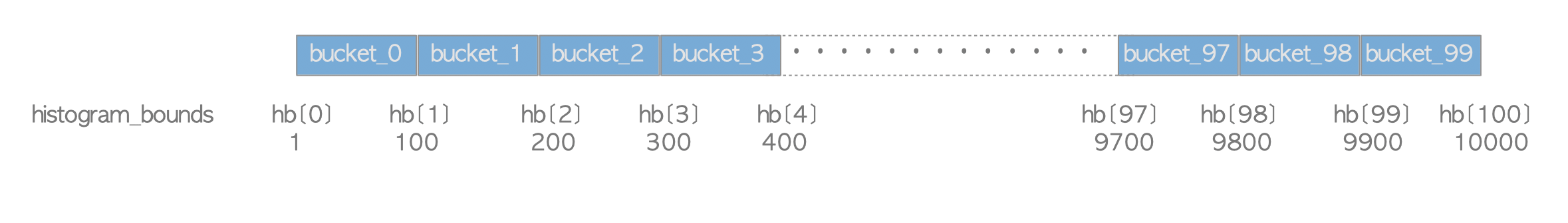
Figure 3.7. Buckets and histogram_bounds.
Next, the calculation of the selectivity will be shown using the example in this subsection. The query has a WHERE clause ‘$\text{data} \lt= 240$’ and the value 240 is in the second bucket. In this case, the selectivity can be derived by applying linear interpolation. Thus, the selectivity of the column ‘data’ in this query is calculated using the following equation:
$$ \begin{align} \text{Selectivity} &= \frac{2 + (240-\text{hb[2]})/(\text{hb[3]} - \text{hb[2]})}{100} \\ &= \frac{2 + (240-200) / (300-200)}{100} = \frac{2 + 40/100}{100} \\ &= 0.024 \tag{6} \end{align} $$Thus, according to (1),(3),(4) and (6),
$$ \begin{align} \text{'index cpu cost'} &= 0.024 \times 10000 \times (0.005 + 0.0025) = 1.8 \tag{7} \\ \text{'table cpu cost'} &= 0.024 \times 10000 \times 0.01 = 2.4 \tag{8} \\ \text{'index IO cost'} &= \mathrm{ceil}(0.024 \times 30) \times 4.0 = 4.0 \tag{9} \end{align} $$$ \text{’table IO cost’} $ is defined by the following equation:
$$ \begin{align} \text{'table IO cost'} = \text{max_IO_cost} + \text{indexCorrelation}^2 \times (\text{min_IO_cost} - \text{max_IO_cost}) \end{align} $$$ \text{max_IO_cost} $ is the worst case of the IO cost, that is, the cost of randomly scanning all table pages; this cost is defined by the following equation:
$$ \begin{align} \text{max_IO_cost} = N_{page} \times \text{random_page_cost} \end{align} $$In this case, according to (2), $ N_{page} = 45 $, and thus
$$ \begin{align} \text{max_IO_cost} = 45 \times 4.0 = 180.0 \tag{10} \end{align} $$$ \text{min_IO_cost} $ is the best case of the IO cost, that is, the cost of sequentially scanning the selected table pages; this cost is defined by the following equation:
$$ \begin{align} \text{min_IO_cost} = 1 \times \text{random_page_cost} + (\mathrm{ceil}(\text{Selectivity} \times N_{page}) - 1) \times \text{seq_page_cost} \end{align} $$In this case,
$$ \begin{align} \text{min_IO_cost} = 1 \times 4.0 + (\mathrm{ceil}(0.024 \times 45)) - 1) \times 1.0 = 5.0 \tag{11} \end{align} $$$ \text{indexCorrelation} $ is described in detail in below, and in this example,
$$ \begin{align} \text{indexCorrelation} = 1.0 \tag{12} \end{align} $$Thus, according to (10),(11) and (12),
$$ \begin{align} \text{'table IO cost'} = 180.0 + 1.0^2 \times (5.0 - 180.0) = 5.0 \tag{13} \end{align} $$Finally, according to (7),(8),(9) and (13),
$$ \begin{align} \text{'run cost'} = (1.8 + 2.4) + (4.0 + 5.0) = 13.2 \tag{14} \end{align} $$Index correlation is a statistical correlation between the physical row ordering and the logical ordering of the column values (cited from the official document). This ranges from -1 to +1. To understand the relation between the index scan and the index correlation, a specific example is shown below.
The table ’tbl_corr’ has five columns: two columns are text type and three columns are integer type. The three integer columns store numbers from 1 to 12. Physically, tbl_corr is composed of three pages, and each page has four tuples. Each integer type column has an index with a name such as index_col_asc and so on.
testdb=# \d tbl_corr
    Table "public.tbl_corr"
  Column  |  Type   | Modifiers
----------+---------+-----------
 col      | text    |
 col_asc  | integer |
 col_desc | integer |
 col_rand | integer |
 data     | text    |
Indexes:
    "tbl_corr_asc_idx" btree (col_asc)
    "tbl_corr_desc_idx" btree (col_desc)
"tbl_corr_rand_idx" btree (col_rand)testdb=# SELECT col,col_asc,col_desc,col_rand
testdb-# FROM tbl_corr;
col | col_asc | col_desc | col_rand
----------+---------+----------+----------
Tuple_1 | 1 | 12 | 3
Tuple_2 | 2 | 11 | 8
Tuple_3 | 3 | 10 | 5
Tuple_4 | 4 | 9 | 9
Tuple_5 | 5 | 8 | 7
Tuple_6 | 6 | 7 | 2
Tuple_7 | 7 | 6 | 10
Tuple_8 | 8 | 5 | 11
Tuple_9 | 9 | 4 | 4
Tuple_10 | 10 | 3 | 1
Tuple_11 | 11 | 2 | 12
Tuple_12 | 12 | 1 | 6
(12 rows)The index correlations of these columns are shown below:
testdb=# SELECT tablename,attname, correlation FROM pg_stats WHERE tablename = 'tbl_corr';
 tablename | attname  | correlation
-----------+----------+-------------
 tbl_corr  | col_asc  |           1
 tbl_corr  | col_desc |          -1
 tbl_corr  | col_rand |    0.125874
(3 rows)
When the following query is executed, PostgreSQL reads only the first page because all of the target tuples are stored in the first page. See Figure 3.8(a).
testdb=# SELECT * FROM tbl_corr WHERE col_asc BETWEEN 2 AND 4;On the other hand, when the following query is executed, PostgreSQL has to read all pages. See Figure 3.8(b).
testdb=# SELECT * FROM tbl_corr WHERE col_rand BETWEEN 2 AND 4;In this way, the index correlation is a statistical correlation that reflects the impact of random access caused by the discrepancy between the index ordering and the physical tuple ordering in the table when estimating the index scan cost.
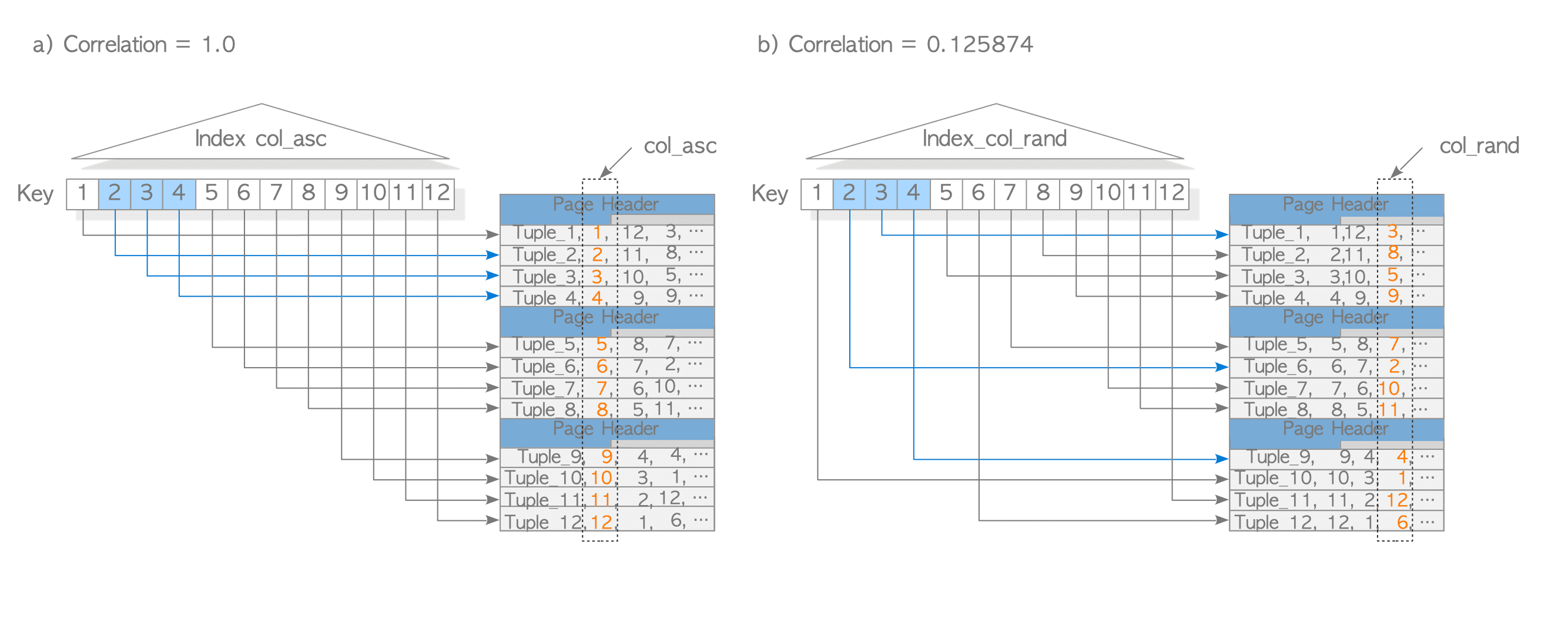
Figure 3.8. Index correlation.
3.2.2.3. Total Cost
According to (3) and (14),
$$ \begin{align} \text{'total cost'} = 0.285 + 13.2 = 13.485 \tag{15} \end{align} $$For confirmation, the result of the EXPLAIN command of the above SELECT query is shown below:
|
|
In Line 4, we can find that the start-up and total costs are 0.29 and 13.49, respectively, and it is estimated that 240 rows (tuples) will be scanned.
In Line 5, an index condition ‘$\text{Index} \text{Cond}:(\text{data} \lt= 240)$’ of the index scan is shown. More precisely, this condition is called an access predicate, and it expresses the start and stop conditions of the index scan.
According to this post, EXPLAIN command in PostgreSQL does not distinguish between the access predicate and index filter predicate. Therefore, when analyzing the output of EXPLAIN, it is important to consider both the index conditions and the estimated value of rows.
The default values of seq_page_cost and random_page_cost are 1.0 and 4.0, respectively.
This means that PostgreSQL assumes that the random scan is four times slower than the sequential scan. In other words, the default value of PostgreSQL is based on using HDDs.
On the other hand, in recent days, the default value of random_page_cost is too large because SSDs are mostly used. If the default value of random_page_cost is used despite using an SSD, the planner may select ineffective plans. Therefore, when using an SSD, it is better to change the value of random_page_cost to 1.0.
This blog reported the problem when using the default value of random_page_cost.
3.2.3. Sort
The sort path is used for sorting operations, such as ORDER BY, the preprocessing of merge join operations, and other functions. The cost of sorting is estimated using the cost_sort() function.
In the sorting operation, if all tuples to be sorted can be stored in work_mem, the quicksort algorithm is used. Otherwise, a temporary file is created and the file merge sort algorithm is used.
The start-up cost of the sort path is the cost of sorting the target tuples. Therefore, the cost is $ O(N_{sort} \times \log_2(N_{sort})) $, where $ N_{sort} $ is the number of the tuples to be sorted. The run cost of the sort path is the cost of reading the sorted tuples. Therefore the cost is $ O(N_{sort}) $.
In this subsection, we explore how to estimate the sorting cost of the following query. Assume that this query will be sorted in work_mem, without using temporary files.
testdb=# SELECT id, data FROM tbl WHERE data <= 240 ORDER BY id;In this case, the start-up cost is defined in the following equation:
$$ \begin{align} \text{'start-up cost'} = C + \text{comparison_cost} \times N_{sort} \times \log_2(N_{sort}) \end{align} $$where:
- $ C $ is the total cost of the last scan, that is, the total cost of the index scan; according to (15), it is 13.485.
- $ N_{sort} $ is the number of tuples to be sorted. In this case, it is 240.
- $ \text{comparison_cost} $ is defined in $ 2 \times \text{cpu_operator_cost} $.
Therefore, the $ \text{start-up cost} $ is calculated as follows:
$$ \begin{align} \text{'start-up cost'} = 13.485 + (2 \times 0.0025) \times 240.0 \times \log_2(240.0) = 22.973 \end{align} $$The $ \text{run cost} $ is the cost of reading sorted tuples in the memory. Therefore,
$$ \begin{align} \text{'run cost'} = \text{cpu_operator_cost} \times N_{sort} = 0.0025 \times 240 = 0.6 \end{align} $$Finally,
$$ \begin{align} \text{'total cost'} = 22.973 + 0.6 = 23.573 \end{align} $$For confirmation, the result of the EXPLAIN command of the above SELECT query is shown below:
|
|
In line 4, we can find that the start-up cost and total cost are 22.97 and 23.57, respectively.
3.2.4. Cardinality Estimation
Previous discussions assumed that Selectivity could be determined with accuracy. In reality, however, selectivity estimation has been one of the most persistent and challenging problems in database systems, from the early days to the present.
3.2.4.1. Selectivity vs. Cardinality
While PostgreSQL internally uses Selectivity, the database field generally focuses on Cardinality. Cardinality is an integer and the relationship between Selectivity and Cardinality is defined as:
$$\text{Selectivity} = \frac{\text{Cardinality}}{N_{\text{tuple}}}$$
Where $N_{\text{tuple}}$ is the total number of tuples (rows) in the table. Cardinality will be used primarily going forward.
3.2.4.2. Demonstrating the Difficulty of Cardinality Estimation
Let’s use a concrete example to illustrate the difficulty of Cardinality Estimation.
Consider a database of 100 villagers.
The residents table records their age category (under18, young, middle, elder) and driver’s license status (none, standard, gold).
(Here, “gold license” is a term used in Japan for a license issued to drivers who have been accident- and violation-free for five years.)
Database Setup
The table structure is defined as follows:
testdb=# CREATE TYPE license AS ENUM ('none', 'standard', 'gold');
CREATE TYPE
testdb=# CREATE TYPE age AS ENUM ('under18', 'young', 'middle', 'elder');
CREATE TYPE

testdb=# CREATE TABLE residents (id int, name text, license license, age age);
CREATE TABBLE

testdb=# \d residents
Table "public.residents"
 Column  |  Type   | Collation | Nullable | Default
---------+---------+-----------+----------+---------
 id      | integer |           |          |
 name    | text    |           |          |
 license | license |           |          |
 age     | age     |           |          |
The residents.csv is here:
testdb=# COPY residents FROM '/usr/local/pgsql/residents.csv' (FORMAT csv);
COPY 100
testdb=# ANALYZE;
ANALYZE
Frequency Distribution
The Most Common Values (MCVs) and their frequencies for the age and license columns are shown below:
-
Age Category Frequency Distribution:
testdb=# SELECT most_common_vals, most_common_freqs FROM pg_stats WHERE tablename = 'residents' AND attname='age';
       most_common_vals       |  most_common_freqs
------------------------------+---------------------
 {middle,young,under18,elder} | {0.35,0.25,0.2,0.2}
(1 row)
Age Category Frequency Distribution Corresponding Residents (100 total) under18 0.2 20 people young 0.25 25 people middle 0.35 35 people elder 0.2 20 people -
License Status Frequency Distribution:
testdb=# SELECT most_common_vals, most_common_freqs FROM pg_stats WHERE tablename = 'residents' AND attname='license';
   most_common_vals   | most_common_freqs
----------------------+-------------------
 {standard,none,gold} | {0.55,0.4,0.05}
(1 row)
License Status Frequency Distribution Corresponding Residents (100 total) none 0.4 40 people standard 0.55 55 people gold 0.05 5 people
3.2.4.3. Initial Estimation Failure (Without Correlation Awareness)
Next, a SELECT statement is executed to retrieve residents who are under18 and have no license (none). EXPLAIN ANALYZE is used to compare the planner’s estimated value with the actual value.
testdb=# EXPLAIN (ANALYZE TRUE, TIMING FALSE, BUFFERS FALSE)
testdb-# 	 	  SELECT * FROM residents WHERE age = 'under18' AND license = 'none';
                                      QUERY PLAN
--------------------------------------------------------------------------------------
 Seq Scan on residents  (cost=0.00..2.50 rows=8 width=18) (actual rows=20.00 loops=1)
   Filter: ((age = 'under18'::age) AND (license = 'none'::license))
   Rows Removed by Filter: 80
 Planning Time: 0.183 ms
 Execution Time: 0.048 ms
(8 rows)
The estimated value is 8, but the actual value is 20.
The actual value of 20 is correct because (at least in the author’s home country, Japan) individuals under 18 cannot obtain a driver’s license. Therefore, all 20 residents in the under18 age group must have no license.
3.2.4.4. The Root Cause: Assuming Independence
The PostgreSQL planner estimated 8 by simply multiplying the proportion of under18 (0.2) and the proportion of none (0.4), assuming the columns were independent: $(0.2 \times 0.4) \times 100 = 0.08 \times 100 = 8$.
Not just PostgreSQL, but the planners of many RDBMSs calculate Cardinality (and thus Selectivity) by assuming that columns are mutually independent unless otherwise specified, without considering the correlation between them. Consequently, the stronger the correlation between columns, the more the planner’s estimation degrades.
There is no complete solution to Cardinality Estimation, and it remains an active area of research.
3.2.4.5. A Partial Solution: Extended Statistics
Despite this situation, partial solutions do exist. For example, PostgreSQL introduced support for extended statistics in Version 13.
By using the CREATE STATISTICS statement, we can store the correlation between the age and license` columns in a new statistic, stat_residents. The planner can then use stat_residents for cardinality estimation, avoiding the assumption of column independence.
testdb=# CREATE STATISTICS stat_residents (mcv) ON license, age FROM residents;
CREATE STATISTICS
testdb=# ANALYZE;
ANALYZE
After creating and analyzing the extended statistics, let’s examine the estimation results for residents in the under18 age group:
-
age = ‘under18’ AND license = ’none’
testdb=# EXPLAIN (ANALYZE TRUE, TIMING FALSE, BUFFERS FALSE) testdb-# SELECT * FROM residents WHERE age = 'under18' AND license = 'none'; QUERY PLAN --------------------------------------------------------------------------------------- Seq Scan on residents (cost=0.00..2.50 rows=20 width=18) (actual rows=20.00 loops=1) Filter: ((age = 'under18'::age) AND (license = 'none'::license)) Rows Removed by Filter: 80 Planning Time: 0.515 ms Execution Time: 0.049 ms (8 rows) -
age = ‘under18’ AND license = ‘standard’
testdb=# EXPLAIN (ANALYZE TRUE, TIMING FALSE, BUFFERS FALSE) testdb-# SELECT * FROM residents WHERE age = 'under18' AND license = 'standard'; QUERY PLAN ------------------------------------------------------------------------------------- Seq Scan on residents (cost=0.00..2.50 rows=1 width=18) (actual rows=0.00 loops=1) Filter: ((age = 'under18'::age) AND (license = 'standard'::license)) Rows Removed by Filter: 100 Planning Time: 0.538 ms Execution Time: 0.073 ms (6 rows) -
age = ‘under18’ AND license = ‘gold’
testdb=# EXPLAIN (ANALYZE TRUE, TIMING FALSE, BUFFERS FALSE)
testdb-# 	 	  SELECT * FROM residents WHERE age = 'under18' AND license = 'gold';
                                     QUERY PLAN
-------------------------------------------------------------------------------------
 Seq Scan on residents  (cost=0.00..2.50 rows=1 width=18) (actual rows=0.00 loops=1)
   Filter: ((age = 'under18'::age) AND (license = 'gold'::license))
   Rows Removed by Filter: 100
 Planning Time: 0.112 ms
 Execution Time: 0.053 ms
(6 rows)
For the under18 age group, the estimated and actual values for “no license” are 20.
The estimated values for “standard” and “gold” are 1, while the actual values are 0. (The estimated value of 1 is likely due to rounding errors.)
PostgreSQL’s Extended Statistics created via CREATE STATISTICS can only be configured for columns belonging to a single table.
Unfortunately, this feature cannot be applied to joins involving multiple tables.
This limitation means that the accuracy of Cardinality Estimation during JOIN operations remains significantly poor.
In fact, cardinality estimation across multiple tables is a major challenge. While extensive research has been conducted, a practical, universally applicable solution is yet to be achieved. This area continues to be a frontier in RDBMS research.