3.6. Creating the Plan Tree of Multiple-Table Query
In this section, the process of creating a plan tree of a multiple-table query is explained.
3.6.1. Preprocessing
The subquery_planner() function defined in planner.c invokes preprocessing. The preprocessing for single-table queries has already been described in Section 3.3.1. In this subsection, the preprocessing for a multiple-table query will be described. However, only some parts will be described, as there are many.
-
Planning and Converting CTE
If there are WITH lists, the planner processes each WITH query by the SS_process_ctes() function. -
Pulling Subqueries Up
If the FROM clause has a subquery and it does not have GROUP BY, HAVING, ORDER BY, LIMIT or DISTINCT clauses, and also it does not use INTERSECT or EXCEPT, the planner converts to a join form by the pull_up_subqueries() function.
For example, the query shown below which contains a subquery in the FROM clause can be converted to a natural join query. Needless to say, this conversion is done in the query tree.$$ \Downarrow $$testdb=# SELECT * FROM tbl_a AS a, (SELECT * FROM tbl_b) as b WHERE a.id = b.id;testdb=# SELECT * FROM tbl_a AS a, tbl_b as b WHERE a.id = b.id; -
Transforming an Outer Join to an Inner Join
The planner transforms an outer join query to an inner join query if possible.
3.6.2. Getting the Cheapest Path
To get the optimal plan tree, the planner has to consider all the combinations of indexes and join methods. This is a very expensive process and it will be infeasible if the number of tables exceeds a certain level due to a combinatorial explosion. Fortunately, if the number of tables is smaller than around 12, the planner can get the optimal plan by applying dynamic programming. Otherwise, the planner uses the genetic algorithm. Refer to the below.
When a query joining many tables is executed, a huge amount of time will be needed to optimize the query plan. To deal with this situation, PostgreSQL implements an interesting feature: the Genetic Query Optimizer.
This is a kind of approximate algorithm to determine a reasonable plan within a reasonable time. Hence, in the query optimization stage, if the number of the joining tables is higher than the threshold specified by the parameter geqo_threshold (the default is 12), PostgreSQL generates a query plan using the genetic algorithm.
Determination of the optimal plan tree by dynamic programming can be explained by the following steps:
-
Level = 1
Get the cheapest path for each table. The cheapest path is stored in the respective RelOptInfo. -
Level = 2
Get the cheapest path for each combination of two tables.
For example, if there are two tables, A and B, get the cheapest join path of tables A and B. This is the final answer.
In the following, the RelOptInfo of two tables is represented by {A, B}.
If there are three tables, get the cheapest path for each of {A, B}, {A, C}, and {B, C}. -
Level = 3 and higher
Continue the same process until the level that equals the number of tables is reached.
This way, the cheapest paths of the partial problems are obtained at each level and are used to get the upper level’s calculation. This makes it possible to calculate the cheapest plan tree efficiently.
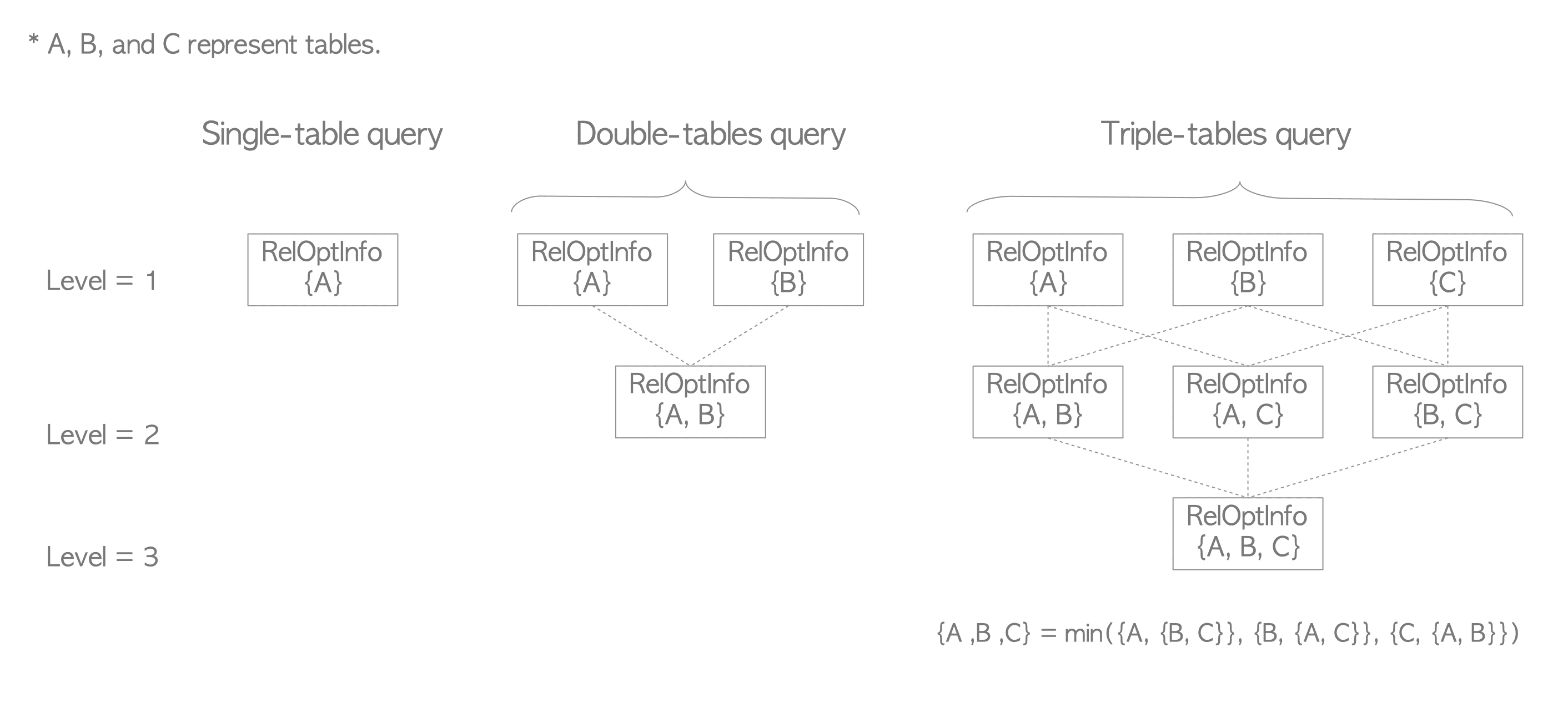
Figure 3.34. How to get the cheapest access path using dynamic programming.
In the following, the process of how the planner gets the cheapest plan of the following query is described.
testdb=# \d tbl_a
     Table "public.tbl_a"
 Column |  Type   | Modifiers
--------+---------+-----------
 id     | integer | not null
 data   | integer |
Indexes:
    "tbl_a_pkey" PRIMARY KEY, btree (id)

testdb=# \d tbl_b
     Table "public.tbl_b"
 Column |  Type   | Modifiers
--------+---------+-----------
 id     | integer |
 data   | integer |

testdb=# SELECT * FROM tbl_a AS a, tbl_b AS b WHERE a.id = b.id AND b.data < 400;
3.6.2.1. Processing in Level 1
In Level 1, the planner creates a RelOptInfo structure and estimates the cheapest costs for each relation in the query. The RelOptInfo structures are added to the simple_rel_array of the PlannerInfo of this query.
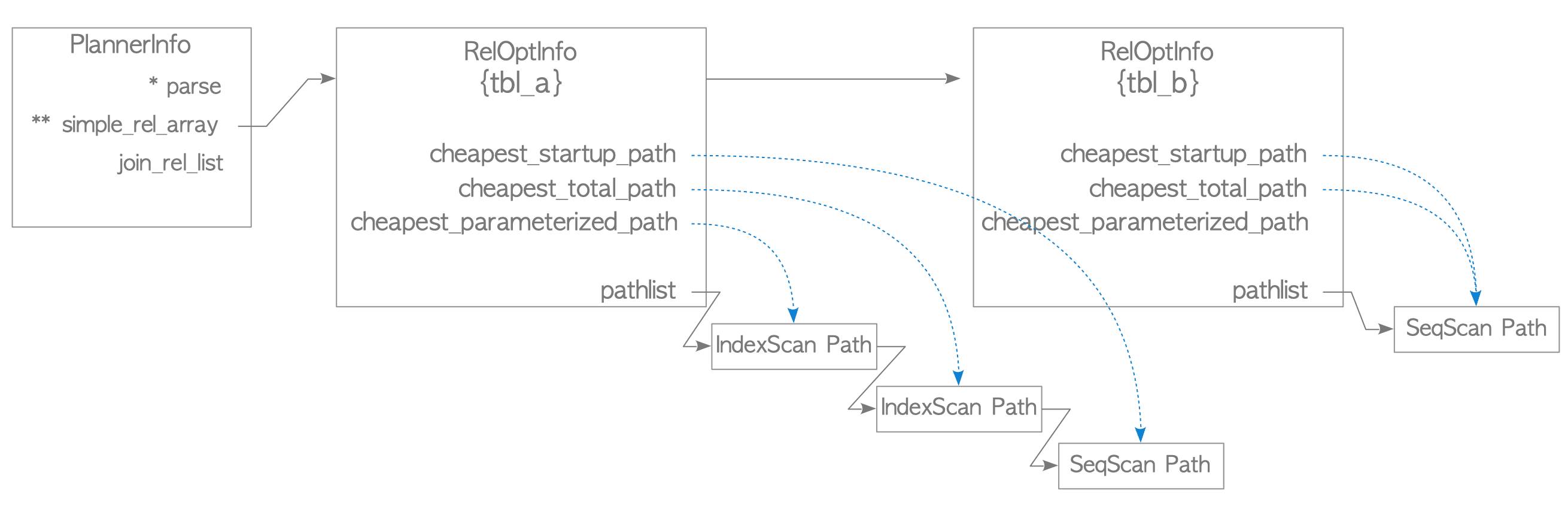
Figure 3.35. The PlannerInfo and RelOptInfo after processing in Level 1.
The RelOptInfo of tbl_a has three access paths, which are added to the pathlist of the RelOptInfo. Each access path is linked to a cheapest cost path: the cheapest start-up (cost) path, the cheapest total (cost) path, and the cheapest parameterized (cost) path. The cheapest start-up and total cost paths are obvious, so the cost of the cheapest parameterized index scan path will be described.
As described in Section 3.5.1.3, the planner considers the use of the parameterized path for the indexed nested loop join (and rarely the indexed merge join with an outer index scan). The cheapest parameterized cost is the cheapest cost of the estimated parameterized paths.
The RelOptInfo of tbl_b only has a sequential scan access path because tbl_b does not have a related index.
3.6.2.2. Processing in Level 2
In level 2, a RelOptInfo structure is created and added to the join_rel_list of the PlannerInfo. Then, the costs of all possible join paths are estimated, and the best access path, whose total cost is the cheapest, is selected. The RelOptInfo stores the best access path as the cheapest total cost path. See Figure 3.36.
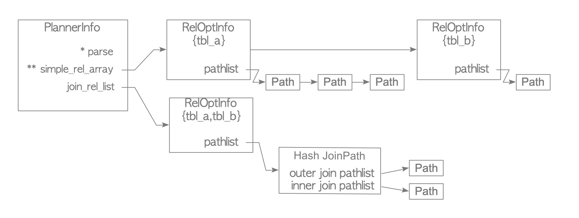
Figure 3.36. The PlannerInfo and RelOptInfo after processing in Level 2.
Table 3.1 shows all combinations of join access paths in this example. The query of this example is an equi-join type, so all three join methods are estimated. For convenience, some notations of access paths are introduced:
-
SeqScanPath(table) means the sequential scan path of table.
-
Materialized->SeqScanPath(table) means the materialized sequential scan path of a table.
-
IndexScanPath(table, attribute) means the index scan path by the attribute of the a table.
-
ParameterizedIndexScanPath(table, attribute1, attribute2) means the parameterized index path by the attribute1 of the table, and it is parameterized by attribute2 of the outer table.
| Outer Path | Inner Path | ||
|---|---|---|---|
| Nested Loop Join | 1 | SeqScanPath(tbl_a) | SeqScanPath(tbl_b) |
| 2 | SeqScanPath(tbl_a) | Materialized->SeqScanPath(tbl_b) | Materialized nested loop join |
| 3 | IndexScanPath(tbl_a,id) | SeqScanPath(tbl_b) | Nested loop join with outer index scan |
| 4 | IndexScanPath(tbl_a,id) | Materialized->SeqScanPath(tbl_b) | Materialized nested loop join with outer index scan |
| 5 | SeqScanPath(tbl_b) | SeqScanPath(tbl_a) | |
| 6 | SeqScanPath(tbl_b) | Materialized->SeqScanPath(tbl_a) | Materialized nested loop join |
| 7 | SeqScanPath(tbl_b) | ParametalizedIndexScanPath(tbl_a, id, tbl_b.id) | Indexed nested loop join |
| Merge Join | 1 | SeqScanPath(tbl_a) | SeqScanPath(tbl_b) |
| 2 | IndexScanPath(tbl_a,id) | SeqScanPath(tbl_b) | Merge join with outer index scan |
| 3 | SeqScanPath(tbl_b) | SeqScanPath(tbl_a) | |
| Hash Join | 1 | SeqScanPath(tbl_a) | SeqScanPath(tbl_b) |
| 2 | SeqScanPath(tbl_b) | SeqScanPath(tbl_a) | |
For example, in the nested loop join, seven join paths are estimated. The first one indicates that the outer and inner paths are the sequential scan paths of tbl_a and tbl_b, respectively. The second indicates that the outer path is the sequential scan path of tbl_a and the inner path is the materialized sequential scan path of tbl_b. And so on.
The planner finally selects the cheapest access path from the estimated join paths, and the cheapest path is added to the pathlist of the RelOptInfo {tbl_a,tbl_b}. See Figure 3.36.
In this example, as shown in the result of EXPLAIN below, the planner selects the hash join whose inner and outer tables are tbl_b and tbl_c.
testdb=# EXPLAIN  SELECT * FROM tbl_b AS b, tbl_c AS c WHERE c.id = b.id AND b.data < 400;
                              QUERY PLAN
----------------------------------------------------------------------
 Hash Join  (cost=90.50..277.00 rows=400 width=16)
   Hash Cond: (c.id = b.id)
   ->  Seq Scan on tbl_c c  (cost=0.00..145.00 rows=10000 width=8)
   ->  Hash  (cost=85.50..85.50 rows=400 width=8)
         ->  Seq Scan on tbl_b b  (cost=0.00..85.50 rows=400 width=8)
               Filter: (data < 400)
(6 rows)
3.6.3. Getting the Cheapest Path of a Triple-Table Query
Obtaining the cheapest path of a query involving three tables is as follows:
testdb=# \d tbl_a
     Table "public.tbl_a"
 Column |  Type   | Modifiers
--------+---------+-----------
 id     | integer |
 data   | integer |

testdb=# \d tbl_b
     Table "public.tbl_b"
 Column |  Type   | Modifiers
--------+---------+-----------
 id     | integer |
 data   | integer |

testdb=# \d tbl_c
     Table "public.tbl_c"
 Column |  Type   | Modifiers
--------+---------+-----------
 id     | integer | not null
 data   | integer |
Indexes:
    "tbl_c_pkey" PRIMARY KEY, btree (id)

testdb=# SELECT * FROM tbl_a AS a, tbl_b AS b, tbl_c AS c
testdb-# WHERE a.id = b.id AND b.id = c.id AND a.data < 40;-
Level 1:
The planner estimates the cheapest paths of all tables and stores this information in the corresponding RelOptInfo objects: {tbl_a}, {tbl_b}, and {tbl_c}. -
Level 2:
The planner picks all the combinations of pairs of the three tables and estimates the cheapest path for each combination. The planner then stores the information in the corresponding RelOptInfo objects: {tbl_a, tbl_b}, {tbl_b, tbl_c}, and {tbl_a, tbl_c}. -
Level 3:
The planner finally gets the cheapest path using the already obtained RelOptInfo objects.
More precisely, the planner considers three combinations of RelOptInfo objects: {tbl_a, {tbl_b, tbl_c}}, {tbl_b, {tbl_a, tbl_c}}, and {tbl_c, {tbl_a, tbl_b}}, because
The planner then estimates the costs of all possible join paths in them.
In the RelOptInfo onject {tbl_c, {tbl_a, tbl_b}}, the planner estimates all the combinations of tbl_c and the cheapest path of {tbl_a, tbl_b}, which is the hash join whose inner and outer tables are tbl_a and tbl_b, respectively, in this example.
The estimated join paths will contain three kinds of join paths and their variations, such as those shown in the previous subsection, that is, the nested loop join and its variations, the merge join and its variations, and the hash join.
The planner processes the RelOptInfo objects {tbl_a, {tbl_b, tbl_c}} and {tbl_b, {tbl_a, tbl_c}} in the same way and finally selects the cheapest access path from all the estimated paths.
The result of the EXPLAIN command of this query is shown below:
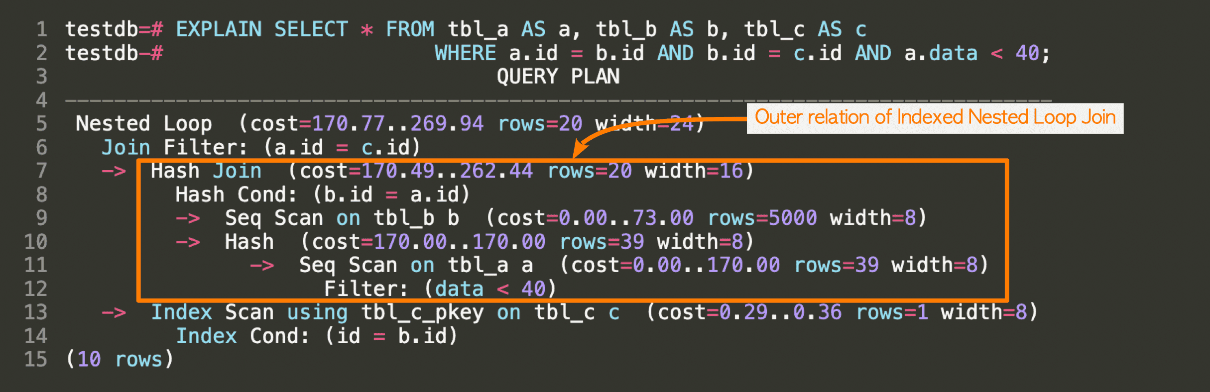
The outermost join is the indexed nested loop join (Line 5). The inner parameterized index scan is shown in line 13, and the outer relation is the result of the hash join whose inner and outer tables are tbl_b and tbl_a, respectively (lines 7-12). Therefore, the executor first executes the hash join of tbl_a and tbl_b and then executes the indexed nested loop join.