3.5.3. Hash Join
Similar to the merge join, the hash join can be only used in natural joins and equi-joins.
The hash join in PostgreSQL behaves differently depending on the sizes of the tables. If the target table is small enough (more precisely, the size of the inner table is 25% or less of the work_mem), it will be a simple two-phase in-memory hash join. Otherwise, the hybrid hash join is used with the skew method.
In this subsection, the execution of both hash joins in PostgreSQL is described.
Discussion of the cost estimation has been omitted because it is complicated. Roughly speaking, the start-up and run costs are $ O(N_{outer} + N_{inner}) $ if assuming there is no conflict when searching and inserting into a hash table.
3.5.3.1. In-Memory Hash Join
In this subsection, the in-memory hash join is described.
This in-memory hash join is processed in the work_mem, and the hash table area is called a batch in PostgreSQL. A batch has hash slots, internally called buckets, and the number of buckets is determined by the ExecChooseHashTableSize() function defined in nodeHash.c; the number of buckets is always $ 2^{n} $, where $ n $ is an integer.
The in-memory hash join has two phases: the build and the probe phases. In the build phase, all tuples of the inner table are inserted into a batch; in the probe phase, each tuple of the outer table is compared with the inner tuples in the batch and joined if the join condition is satisfied.
A specific example is shown to clearly understand this operation. Assume that the query shown below is executed using a hash join.
testdb=# SELECT * FROM tbl_outer AS outer, tbl_inner AS inner WHERE inner.attr1 = outer.attr2;In the following, the operation of a hash join is shown. Refer to Figures 3.26 and 3.27.
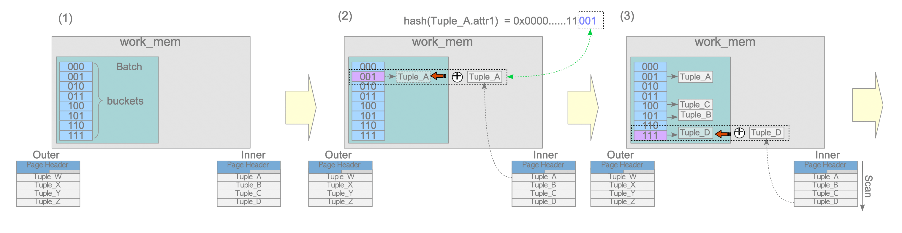
Figure 3.26. The build phase in the in-memory hash join.
-
(1) Create a batch on work_mem.
In this example, the batch has 8 buckets, which means the number of buckets is $ 2^{3} $. -
(2) Insert the first tuple of the inner table into the corresponding bucket of the batch.
The details are as follows:-
Calculate the hash-key of the first tuple’s attribute that is involved in the join condition.
In this example, the hash-key of the attribute ‘attr1’ of the first tuple is calculated using the built-in hash function because the WHERE clause is ‘inner.attr1 = outer.attr2’. -
Insert the first tuple into the corresponding bucket.
Assume that the hash-key of the first tuple is ‘0x000…001’ by binary notatio, which means the last three bits are ‘001’. In this case, this tuple is inserted into the bucket whose key is ‘001’.
-
In this document, this insertion operation to build a batch is represented by this operator: $ \oplus $
- (3) Insert the remaining tuples of the inner table.
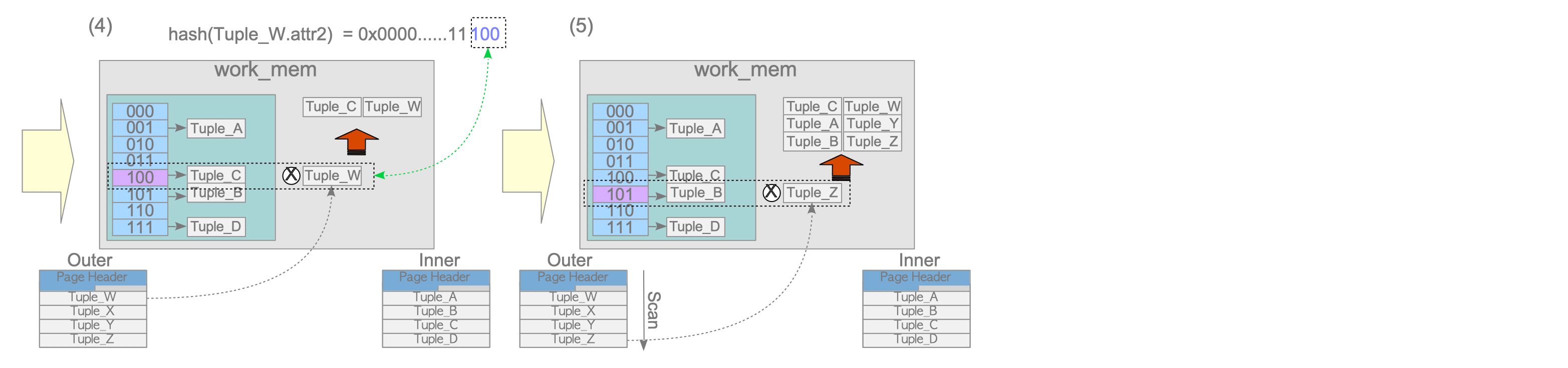
Figure 3.27. The probe phase in the in-memory hash join.
-
(4) Probe the first tuple of the outer table.
The details are as follows:- Calculate the hash key of the first tuple’s attribute that is involved in the join condition of the outer table.
In this example, assume that the hash-key of the first tuple’s attribute ‘attr2’ is ‘0x000…100’; that is, the last three bits are ‘100’. - Compare the first tuple of the outer table with the inner tuples in the batch and join tuples if the join condition is satisfied.
Because the last three bits of the hash-key of the first tuple are ‘100’, the executor retrieves the tuples belonging to the bucket whose key is ‘100’ and compares both values of the respective attributes of the tables specified by the join condition (defined by the WHERE clause).
If the join condition is satisfied, the first tuple of the outer table and the corresponding tuple of the inner table will be joined. Otherwise, the executor does nothing.
In this example, the bucket whose key is ‘100’ has Tuple_C. If the attr1 of Tuple_C is equal to the attr2 of the first tuple (Tuple_W), then Tuple_C and Tuple_W will be joined and saved to memory or a temporary file.
In this document, such operation to probe a batch is represented by the operator: $ \otimes $
- Calculate the hash key of the first tuple’s attribute that is involved in the join condition of the outer table.
-
(5) Probe the remaining tuples of the outer table.
3.5.3.2. Hybrid Hash Join with Skew
When the tuples of the inner table cannot be stored in one batch in work_mem, PostgreSQL uses the hybrid hash join with the skew algorithm, which is a variation based on the hybrid hash join.
First, the basic concept of the hybrid hash join is described. In the first build and probe phases, PostgreSQL prepares multiple batches. The number of batches is the same as the number of buckets, determined by the ExecChooseHashTableSize() function. It is always $ 2^{m} $, where $ m $ is an integer. At this stage, only one batch is allocated in work_mem, and the other batches are created as temporary files. The tuples belonging to these batches are written to the corresponding files and saved using the temporary tuple storage feature.
Figure 3.28 illustrates how tuples are stored in four (= $ 2^{2} $) batches. In this case, which batch stores each tuple is determined by the first two bits of the last 5 bits of the tuple’s hash-key, because the sizes of the buckets and batches are $ 2^{3} $ and $ 2^{2} $, respectively. Batch_0 stores the tuples whose last 5 bits of the hash-key are between ‘00000’ and ‘00111’, Batch_1 stores the tuples whose last 5 bits of the hash-key are between ‘01000’ and ‘01111’ and so on.
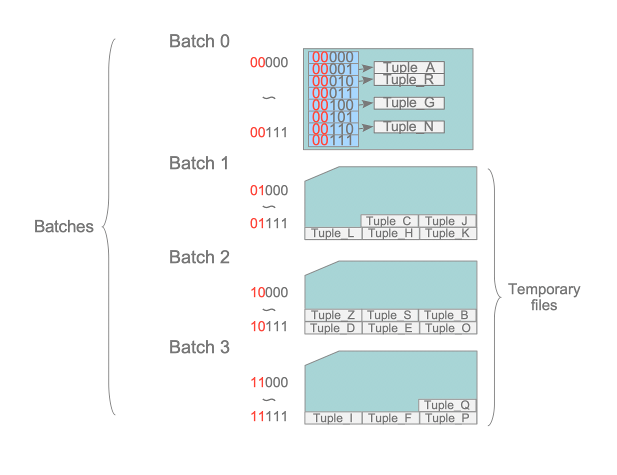
Figure 3.28. Multiple batches in hybrid hash join.
In the hybrid hash join, the build and probe phases are performed the same number of times as the number of batches, because the inner and outer tables are stored in the same number of batches. In the first round of the build and probe phases, not only is every batch created, but also the first batches of both the inner and the outer tables are processed. On the other hand, the processing of the second and subsequent rounds needs writing and reloading to/from the temporary files, so these are costly processes. Therefore, PostgreSQL also prepares a special batch called skew to process many tuples more efficiently in the first round.
The skew batch stores the inner table tuples that will be joined with the outer table tuples whose MCV values of the attribute involved in the join condition are relatively large. However, this explanation may not be easy to understand, so it will be explained using a specific example.
Assume that there are two tables: customers and purchase_history.
- The customers’ table has two attributes: ’name’ and ‘address’.
- the purchase_history table has two attributes: ‘customer_name’ and ‘purchased_item’.
- The customers’ table has 10,000 rows, and the purchase_history table has 1,000,000 rows.
- The top 10% customers have purchased 70% of all items.
Under these assumptions, let us consider how the hybrid hash join with skew performs in the first round when the query shown below is executed.
testdb=# SELECT * FROM customers AS c, purchase_history AS h WHERE c.name = h.customer_name;If the customers’ table is inner and the purchase_history is outer, the top 10% of customers are stored in the skew batch using the MCV values of the purchase_history table. Note that the outer table’s MCV values are referenced to insert the inner table tuples into the skew batch. In the probe phase of the first round, 70% of the tuples of the outer table (purchase_history) will be joined with the tuples stored in the skew batch. This way, the more non-uniform the distribution of the outer table, the more tuples of the outer table can be processed in the first round.
In the following, the working of the hybrid hash join with skew is shown. Refer to Figures 3.29 to 3.32.
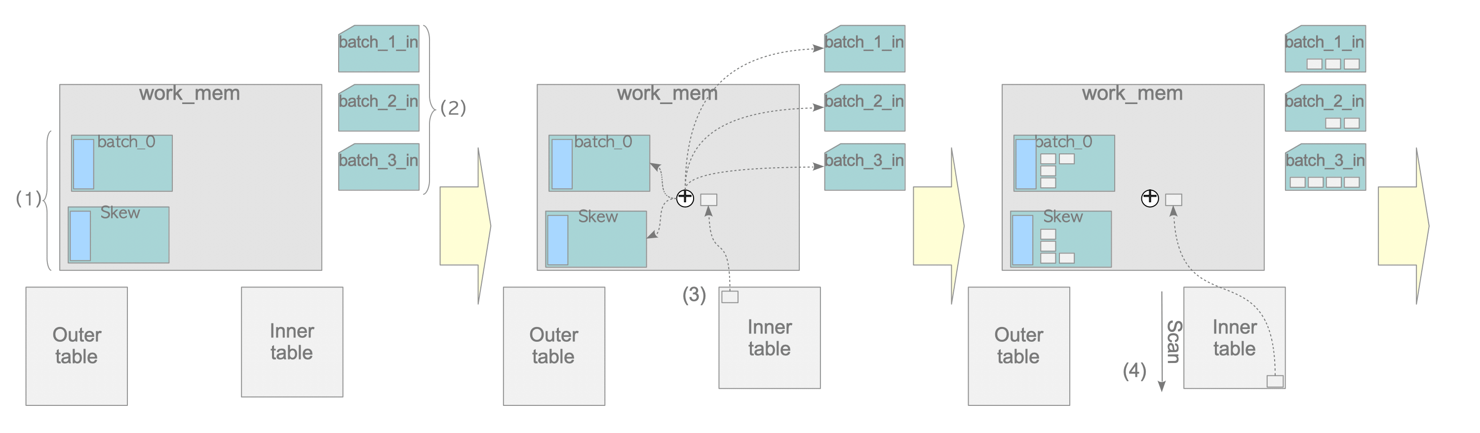
Figure 3.29. The build phase of the hybrid hash join in the first round.
-
(1) Create a batch and a skew batch on work_mem.
-
(2) Create temporary batch files for storing the inner table tuples.
In this example, three batch files are created because the inner table will be divided into four batches. -
(3) Perform the build operation for the first tuple of the inner table.
The detail are described below:- If the first tuple should be inserted into the skew batch, do so. Otherwise, proceed to 2.
In the example explained above, if the first tuple is one of the top 10% customers, it is inserted into the skew batch. - Calculate the hash key of the first tuple and then insert it into the corresponding batch.
- If the first tuple should be inserted into the skew batch, do so. Otherwise, proceed to 2.
-
(4) Perform the build operation for the remaining tuples of the inner table.
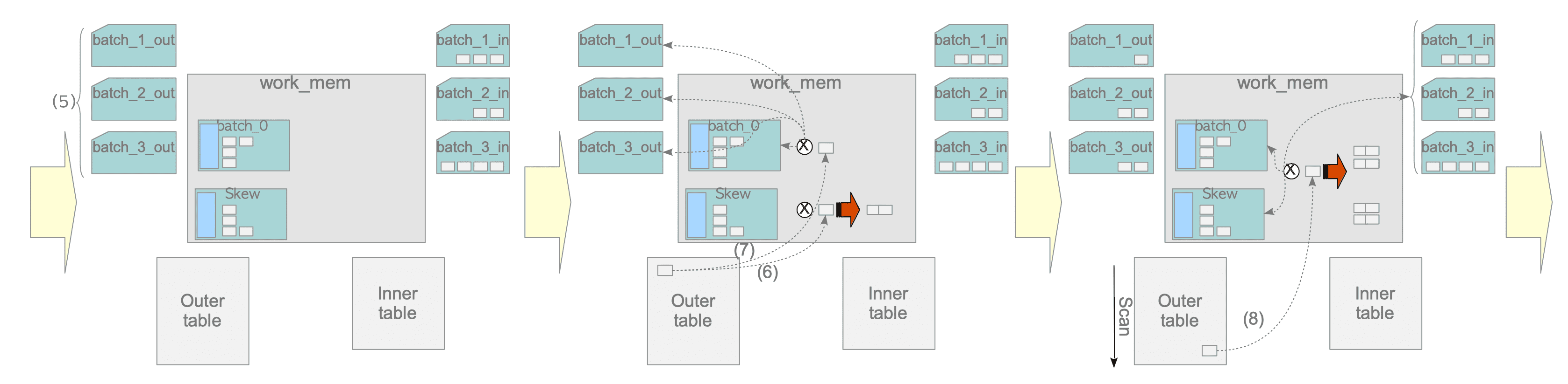
Figure 3.30. The probe phase of the hybrid hash join in the first round.
-
(5) Create temporary batch files for storing the outer table tuples.
-
(6) If the MCV value of the first tuple is large, perform a probe operation with the skew batch. Otherwise, proceed to (7).
In the example explained above, if the first tuple is the purchase data of the top 10% customers, it is compared with the tuples in the skew batch. -
(7) Perform the probe operation of the first tuple.
Depending on the hash-key value of the first tuple, the following process is performed:- If the first tuple belongs to Batch_0, perform the probe operation.
- Otherwise, insert into the corresponding batch.
-
(8) Perform the probe operation from the remaining tuples of the outer table.
Note that, in this example, 70% of the tuples of the outer table have been processed by the skew in the first round without writing and reading to/from temporary files.
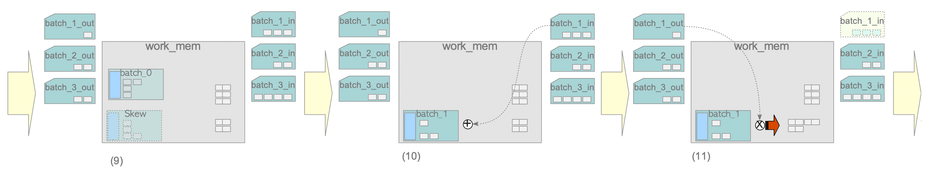
Figure 3.31. The build and probe phases in the second round.
-
(9) Remove the skew batch and clear Batch_0 to prepare the second round.
-
(10) Perform the build operation from the batch file ‘batch_1_in’.
-
(11) Perform the probe operation for tuples which are stored in the batch file ‘batch_1_out’.
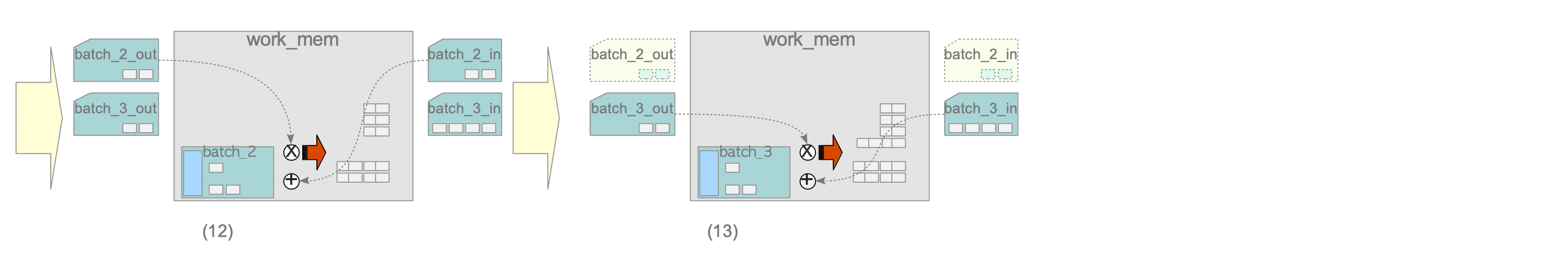
Figure 3.32. The build and probe phases in the third and the last rounds.
-
(12) Perform build and probe operations using batch files ‘batch_2_in’ and ‘batch_2_out’.
-
(13) Perform build and probe operations using batch files ‘batch_3_in’ and ‘batch_3_out’.
3.5.3.3. Index Scans in Hash Join
Hash join in PostgreSQL uses index scans if possible. A specific example is shown below.
|
|
- Line 7: In the probe phase, PostgreSQL uses the index scan when scanning the pgbench_accounts table because there is a condition of the column ‘aid’ which has an index in the WHERE clause.