3.4. Executor Performance
This section describes the basic operation of the Executor during query processing.
It also describes the processing of aggregate functions and the internal processing of table constraints, both of which are important for practical use.
3.4.1. How the Executor Performs
PostgreSQL utilizes the Volcano Model (also known as the Iterator Model) for query execution.
In this model, the executor processes the plan tree by invoking the functions associated with each node. From a data flow perspective, tuples move upward from the leaf nodes to the root.
Each plan node has specific functions responsible for its operation, located in the src/backend/executor/ directory. For example:
- Sequential Scan (SeqScan): Defined in nodeSeqscan.c.
- Index Scan (IndexScan): Defined in nodeIndexscan.c.
- Sort (Sort): Defined in nodeSort.c.
The operation of the executor is best understood by examining the output of the EXPLAIN command, which reflects the structure of the plan tree. Consider the following result from Example 1 (Section 3.3.3.1):
|
|
When analyzing the execution flow, the EXPLAIN output is typically read from the bottom up:
-
Line 6 (SeqScan): The SeqScan node (defined in nodeSeqscan.c) sequentially scans the target table, applies the filter “id < 300”, and passes the resulting tuples upward to the SortNode.
-
Line 4 (Sort): The SortNode (defined in nodeSort.c) receives tuples one by one from its child (the SeqScanNode) and stores them in the work_mem buffer. Once the child node has finished providing tuples, the SortNode performs the sorting operation.
From a control-flow perspective, the executor starts at the SortNode. The SortNode then repeatedly invokes the SeqScan node to obtain tuples. As shown in Figure 3.16, these tuples are collected in memory before the final sort is executed.
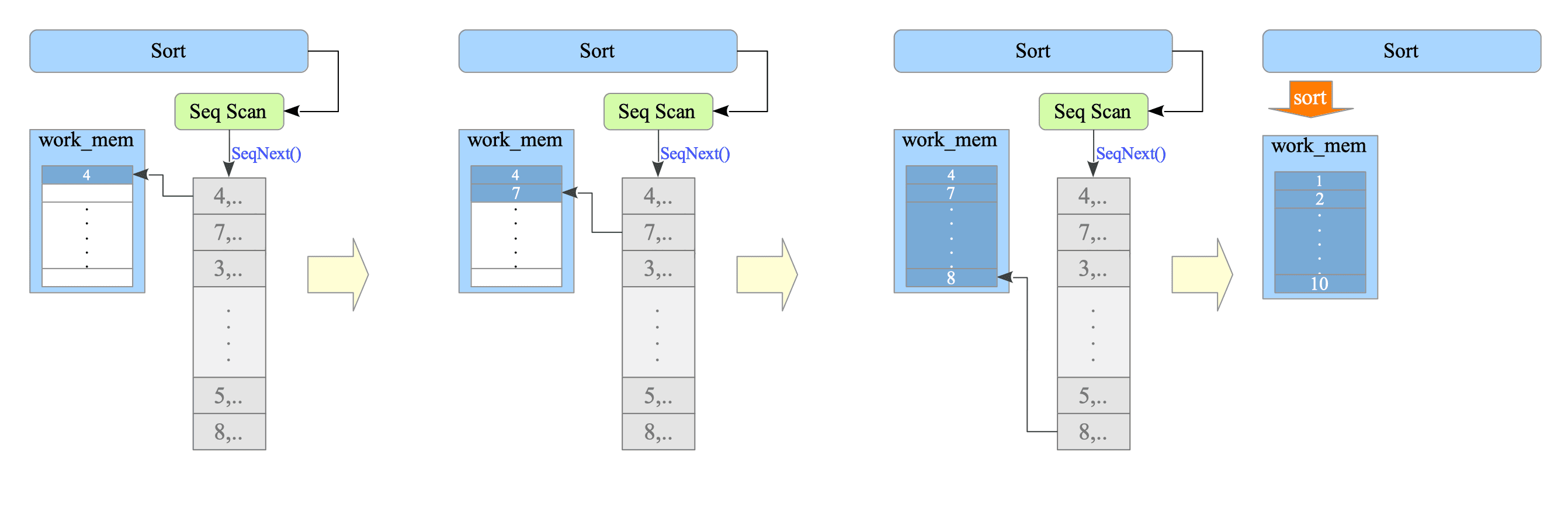
Figure 3.16. Sort Processing in the Executor.
3.4.1.1. Scanning Functions
As mentioned in Section 1.3, data tuples are stored in 8 KB physical blocks. To access a single data tuple, the Executor must traverse many layers, such as Buffer Manager (see Chapter 8) and Concurrency Control (see Chapter 5). Furthermore, the access method differs depending on whether the data block belongs to a table or an index.
The method of accessing a single data tuple by the Executor is highly abstracted, and the complexity of the intermediate layers is hidden.
For example, in the case of a sequential scan, by repeatedly calling the SeqNext() function, rows in a table can be accessed sequentially, taking transactions into account. For an index scan, an index scan can be performed by repeatedly calling the IndexNext() function.
3.4.1.2. Temporary Files
The executor utilizes work_mem and temp_buffers allocated in memory for query processing. However, if a task – such as sorting or hash aggregation — exceeds the available memory, the executor switches to temporary files on disk.
By using the ANALYZE option, the EXPLAIN command executes the query and displays the actual row counts, run time, and memory or disk usage. An example of this is shown below:
|
|
On Line 6, the EXPLAIN ANALYZE output indicates that the executor performed an “external sort” and used a temporary file of 10,000 kB.
Temporary files are created under the $PGDATA/base/pg_tmp subdirectory.
They follow a specific naming convention:
- Temporary File Pattern:
pgsql_tmp[PID].[seq_number]
For instance, a file named ‘pgsql_tmp8903.5’ represents the 6th temporary file (as the sequence number is zero-indexed) created by the Postgres process with PID 8903.
$ ls -la $PGDATA/base/pgsql_tmp*
-rw-------  1 postgres  postgres  10240000 12  4 14:18 pgsql_tmp8903.5
3.4.2. Aggregate Functions
In practice, the efficient calculation of aggregate functions is a critical role of database systems. This section describes how aggregate functions — such as sum, average, and variance — are handled by the executor.
The following table d is used for the examples in this section:
testdb=# CREATE TABLE d (x DOUBLE PRECISION);
CREATE TABLE
testdb=# INSERT INTO d SELECT GENERATE_SERIES(1, 10);
INSERT 0 10
When a sum function is issued, a plan tree is created as shown in Figure 3.17.
testdb=# SELECT sum(x) FROM d;
 sum
-----
  55
(1 row)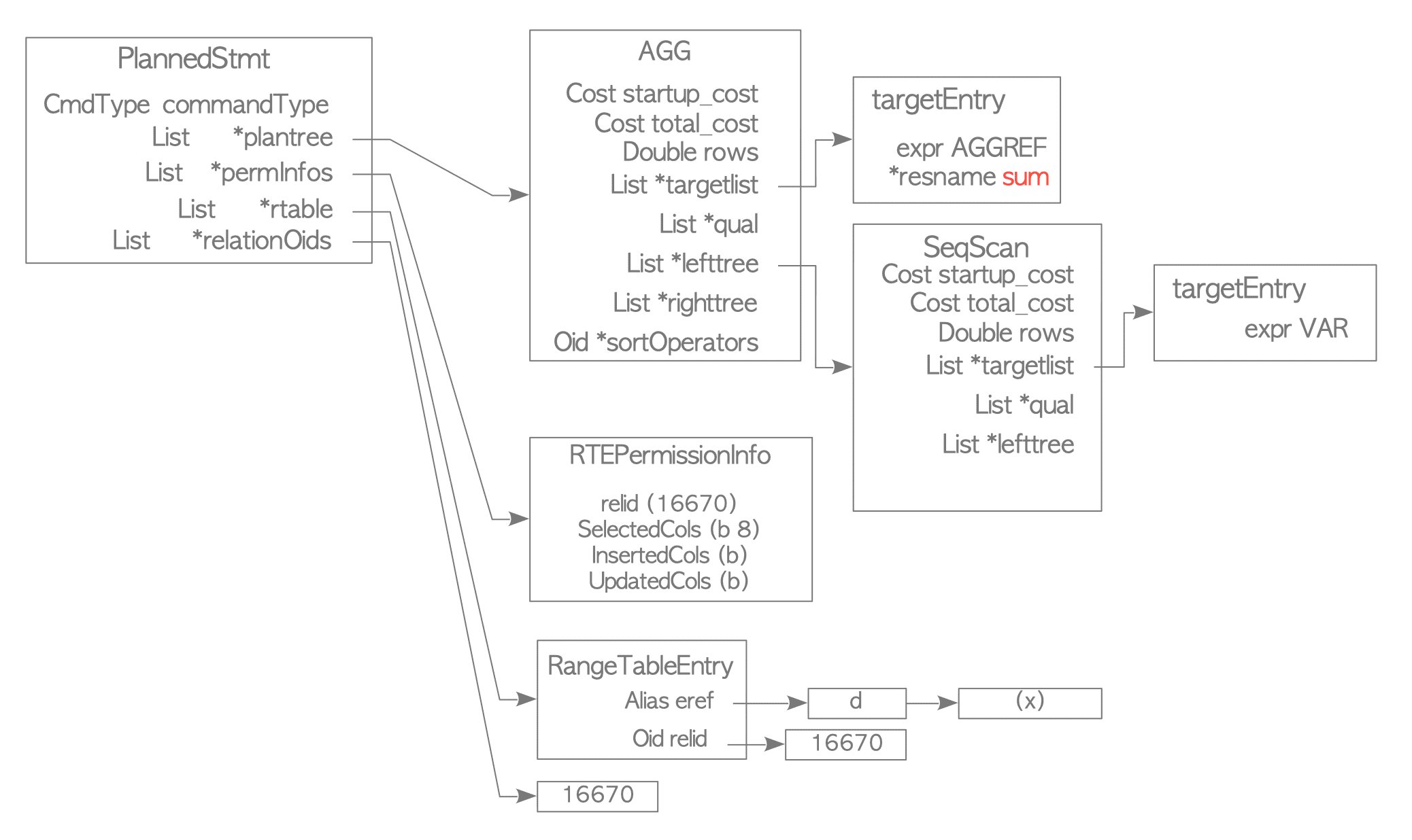
Figure 3.17. A Plan Tree for the Sum Function.
The result of the EXPLAIN command for this query is shown below:
|
|
-
On Line 5: The SeqScan node sequentially scans the target table and passes the values of the target column ‘x’ to the Aggregate node.
-
On Line 4: The Aggregate node receives the data from the SeqScan node and processes it according to the specified aggregate function (e.g., sum, avg, variance, or count).
Figure 3.18 provides an overview of how the aggregate function is processed within the executor.
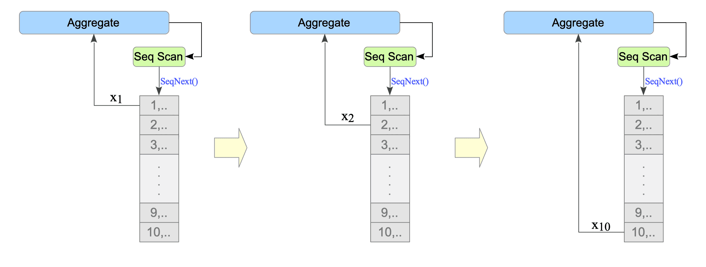
Figure 3.18. Aggregate Function Processing in the Executor.
The following subsections explore the internal processing of aggregate functions using specific examples.
3.4.2.1. Sum and Average
The formulas for the sum $S_{n}$ and average $A_{n}$ are given by:
$$ \begin{align} S_{n} &= \sum_{i=1}^{n} x_{i} \tag{3-16} \\ A_{n} &= \frac{1}{n} \sum_{i=1}^{n} x_{i} = \frac{1}{n} S_{n} \tag{3-17} \end{align} $$where $x_{i}$ epresents the value of the target column in the $i-$th row.
As shown in these formulas, the primary difference between a sum and an average is the final division by the total number of elements, $n$.
Internally, the Aggregate node accumulates the scanned values sequentially.
During the final stage of processing, the node returns the accumulated sum for a sum operation.
For an avg operation, it returns the accumulated sum divided by the count of processed rows ($n$).
The following pseudocode illustrates this logic:
d =[1.0, 2.0, 3.0, 4.0, 5.0, 6.0, 7.0, 8.0, 9.0, 10.0]

N = 0
S = 0

# Seq Scan
for x in d:

    # Aggregate: Sum
    N += 1
    S += x

print("Sum=", S)
print("Avg=", S/N)
3.4.2.2. Variance
For simplicity, variance $V_{n}$ is defined based on the sum of squared deviations from the average:
$$ V_{n} = \sum_{i=1}^{n} (x_{i} - A_{n})^{2} \tag{3-18} $$Based on this definition, PostgreSQL provides two types of variance:
- Sample Variance (var_samp): $\frac{1}{n-1} V_{n}$. This is used when the data represents a sample of a larger population.
- Population Variance (var_pop): $\frac{1}{n} V_{n}$. This is used when the data represents the entire population.
The following examples show the output for both functions:
testdb=# SELECT var_samp(x) FROM d;
     var_samp
-------------------
 9.166666666666666
(1 row)

testdb=# SELECT var_pop(x) FROM d;
 var_pop
---------
    8.25
(1 row)
3.4.2.2.1. One-Pass Variance Calculation (Versions 11 or earlier)
A naive implementation of the variance formula (3−18) requires two passes over the data: the first to calculate the average and a second to calculate the sum of squared differences.
To optimize this, the calculation can be reduced to a single pass using the following formula (For details, refer to the following ):
$$ \begin{align} V_{n} &= \sum_{i=1}^{n} x_{i}^{2} - \frac{1}{n} (S_{n})^{2} \tag{3-19} \\ \end{align} $$This approach allows the executor to calculate the variance iteratively by maintaining running totals for both the sum of the squares ($\sum x^{2}$) and the sum of the values ($S_{n}$).
The following pseudocode illustrates this logic:
d =[1.0, 2.0, 3.0, 4.0, 5.0, 6.0, 7.0, 8.0, 9.0, 10.0]

N = 0
S = 0
X2 = 0

# SeqScan
for x in d:

    # Aggregate: Variance
    N += 1
    S += x
    X2 += x**2

V = X2 - S**2/N

print("V=", V)
print("Var_samp=", V/(N-1))
print("Var_pop=", V/N)3.4.2.2.2. Youngs and Cramer method (Versions 12 or later)
In 2016, a research paper titled “A Closer Look at Variance ImplementationsIn Modern Database Systems” highlighted accuracy limitations in PostgreSQL’s variance calculation.
To address these concerns, a patch was developed in November 2018, leading to the adoption of the Youngs and Cramer method in PostgreSQL version 12. This algorithm provides significantly higher numerical stability and accuracy than the standard single-pass formula1.
The following pseudocode illustrates the implementation of the Youngs and Cramer method:
$$ \begin{cases} V_{1} &= 0 \\ V_{n} &= V_{n-1} + \frac{1}{n(n-1)} (nx_{n} - S_{n})^{2} \tag{3-20} \end{cases} $$Following is the pseudocode of Youngs and Cramer method:
d =[1.0, 2.0, 3.0, 4.0, 5.0, 6.0, 7.0, 8.0, 9.0, 10.0]

N = 0
S = 0
V = 0

# SeqScan
for x in d:

    # Aggregate: Variance
    N += 1
    S += x
    if 1 < N:
        V += (x * N - S)**2 / (N * (N-1))

print("V=", V)
print("Var_samp=", V/(N-1))
print("Var_pop=", V/N)The Youngs and Cramer method is an enhancement of the Welfold’s online method. To understand the derivation of the Youngs and Cramer method, the Welford method is examined first.
Welfold method:
Welford’s method for calculating variance is defined by the following recurrence relation:
$$ V_{n} = V_{n-1} + \frac{n-1}{n} (x_{n} - A_{n-1})^{2} $$The derivation of this relation is as follows:
$$ \begin{align} V_{n} &= \sum_{i=1}^{n} (x_{i} - A_{n})^{2} = \sum_{i=1}^{n-1} (x_{i} - A_{n})^{2} + (x_{n} - A_{n})^{2} \\ &= \sum_{i=1}^{n-1} \left( (x_{i} - \frac{1}{n}((n-1)A_{n-1} + x_{n}) \right)^{2} + \left( (x_{n} - \frac{1}{n}((n-1)A_{n-1} + x_{n}) \right)^{2} \\ &= \sum_{i=1}^{n-1} \left( (x_{i} - A_{n-1}) - \frac{1}{n}(x_{n} - A_{n-1}) \right)^{2} + \left( \frac{1}{n} (nx_{n} - (n-1)A_{n-1} - x_{n} ) \right)^{2} \\ &= \sum_{i=1}^{n-1} \left( (x_{i} - A_{n-1})^{2} - \frac{2(x_{n} - A_{n-1})}{n}(x_{i} - A_{n-1}) + \frac{1}{n^{2}}(x_{n} - A_{n-1})^{2} \right) \\ & \quad + \left( \frac{(n - 1) x_{n} - (n-1) A_{n-1}}{n} \right)^{2} \\ &= \sum_{i=1}^{n-1} (x_{i} - A_{n-1})^{2} - \frac{2(x_{n} - A_{n-1})}{n} \sum_{i=1}^{n-1}(x_{i} - A_{n-1}) + \frac{1}{n^{2}} \sum_{i=1}^{n-1} (x_{n} - A_{n-1})^{2} \\ & \quad + \left( \frac{(n - 1) (x_{n} - A_{n-1})}{n} \right)^{2} \\ &= V_{n-1} - \frac{2(x_{n} - A_{n-1})}{n} \left( \sum_{i=1}^{n-1} x_{i} - (n-1)A_{n-1} \right) + \frac{1}{n^{2}} (n-1) \cdot (x_{n} - A_{n-1})^{2} \\ & \quad + \left( \frac{n-1}{n} \right)^{2} (x_{n} - A_{n-1})^{2} \\ &= V_{n-1} - \frac{2(x_{n} - A_{n-1})}{n} (S_{n-1} - S_{n-1}) + \left( \frac{n-1}{n^{2}} + \left( \frac{n-1}{n}\right)^{2} \right) (x_{n} - A_{n-1})^{2} \\ &= V_{n-1} - \frac{2(x_{n} - A_{n-1})}{n} \cdot 0 + \frac{(n-1) + (n-1)^{2}}{n^{2}} (x_{n} - A_{n-1})^{2} \\ &= V_{n-1} + \frac{(n-1)(1 + (n-1))}{n^{2}} (x_{n} - A_{n-1})^{2} \\ &= V_{n-1} + \frac{n-1}{n} (x_{n} - A_{n-1})^{2} \end{align} $$Youngs and Cramer method:
The Youngs and Cramer method modifies Welford’s method by replacing the average $A_{n-1}$ with the sum $S_{n-1}$ to improve computational efficiency and numerical stability.
The recurrence relation is derived as follows:
$$ \begin{align} V_{n} &= V_{n-1} + \frac{n-1}{n} \left( x_{n} - \frac{S_{n-1}}{n-1} \right)^{2} = V_{n-1} + \frac{n-1}{n} \left( \frac{(n-1)x_{n} - S_{n-1}}{n-1} \right)^{2} \\ &= V_{n-1} + \frac{1}{n(n-1)} ((n-1)x_{n} - S_{n-1})^{2} = V_{n-1} + \frac{1}{n(n-1)} (nx_{n} - x_{n} - (S_{n}- x_{n} ))^{2} \\ &= V_{n-1} + \frac{1}{n(n-1)} (nx_{n} - S_{n})^{2} \end{align} $$3.4.3. Constraints
When PostgreSQL executes an INSERT, UPDATE, or DELETE statement, the Executor checks the constraints defined on the target table.
This section focuses on the following three common constraint types:
- NOT NULL and CHECK constraints
- PRIMARY KEY and UNIQUE constraints
- FOREIGN KEY constraints
To illustrate how PostgreSQL processes these constraints, consider the insertion of a single tuple.
The pseudocode below shows the main flow of the ExecInsert() function:
ExecInsert() @ nodeModifyTable.c

/*
 * Block 1: Validate table constraints
 */
(1) ExecConstraints()@execMain.c       /* Check NOT NULL and CHECK constraints. */

/*
 * Block 2: Insert the heap tuple
 */
(2) table_tuple_insert()@tableam.c     /* Insert the target tuple into the heap table. */

/*
 * Block 3: Insert index tuples and enforce uniqueness
 */
(3) ExecInsertIndexTuples()@execIndexing.c
        for each index:
(4)         index_insert()@indexam.c   /* Insert the corresponding index tuple. */
            if (UNIQUE or PRIMARY KEY index)
(5)             _bt_check_unique()@nbtinsert.c
                                       /* Check whether a conflicting key already exists
                                        * in the B-tree index.
                                        */
/*
 * Block 4: Execute AFTER ROW INSERT triggers
 */
(6) ExecARInsertTriggers()@trigger.c
        for each AFTER INSERT trigger:
(7)         RI_FKey_check_ins()@ri_triggers.c /* Check FOREIGN KEY constraints. */
The major steps are:
- Block 1: Validate table constraints
- (1) ExecConstraints() checks NOT NULL constraints and CHECK constraints.
- Block 2: Insert the heap tuple
- (2) table_tuple_insert() inserts the tuple into the heap table.
- Block 3: Insert index tuples and enforce uniqueness
- (3) ExecInsertIndexTuples() processes all indexes belonging to the table.
- (4) index_insert() inserts the corresponding index tuple into each index.
- (5) _bt_check_unique() checks whether a conflicting key already exists. UNIQUE and PRIMARY KEY constraints are enforced here.
- Block 4: Execute AFTER ROW INSERT triggers
- (6) ExecARInsertTriggers() executes AFTER INSERT triggers.
- (7) RI_FKey_check_ins() checks FOREIGN KEY constraints.
The following sections explain each constraint type in more detail.
3.4.3.1. NOT NULL and CHECK Constraints
PostgreSQL checks these constraints in Block 1.
The ExecConstraints() function checks NOT NULL constraints and CHECK constraints. More precisely, the ExecRelCheck() function evaluates CHECK constraints.
PostgreSQL stores CHECK constraint definitions in the system catalog pg_constraint. PostgreSQL loads these definitions into memory and evaluates the corresponding expressions for each inserted or updated tuple.
The same mechanism applies to UPDATE statements.
3.4.3.2. PRIMARY KEY and UNIQUE Constraints
PostgreSQL checks PRIMARY KEY and UNIQUE constraints in Block 3.
When inserting an index tuple into a UNIQUE index, PostgreSQL checks whether a conflicting key already exists in the index.
The _bt_check_unique() function performs this check for B-tree indexes. Because the function checks the index directly, the check runs in approximately $O(\log n)$ time, where $n$ is the number of index entries.
The same mechanism applies to UPDATE statements.
3.4.3.3. FOREIGN KEY Constraints
PostgreSQL checks FOREIGN KEY constraints in Block 4.
FOREIGN KEY constraints require PostgreSQL to check rows in another table. Therefore, the implementation is more complex than that of the previous two constraint types.
Consider the following tables:
CREATE TABLE tbl_parent (
    id int PRIMARY KEY,
    data text
);

CREATE TABLE tbl_child (
    cid int REFERENCES tbl_parent(id),
    data text
);
Suppose that PostgreSQL executes the following statement:
INSERT INTO tbl_child VALUES (1, 'test');During Block 4, PostgreSQL executes the FOREIGN KEY trigger function.
In versions 18 and earlier, the trigger generates and executes a query similar to the following:
SELECT 1
FROM ONLY "public"."tbl_parent" x
WHERE "id" OPERATOR(pg_catalog.=) $1
FOR KEY SHARE OF x;
This SELECT statement uses FOR KEY SHARE to lock the referenced row. This lock prevents concurrent transactions from deleting the row or modifying the referenced key while PostgreSQL checks the foreign key constraint.
PostgreSQL executes this SELECT statement through the Server Programming Interface (SPI).
Because SPI executes an internal SQL query, PostgreSQL must still perform query processing for the generated query. This processing adds overhead to each FOREIGN KEY check.
Consequently, inserting a single tuple into the child table executes an additional internal SELECT query.
Direct FOREIGN KEY Validation in PostgreSQL 19
PostgreSQL 19 introduces a new execution path for FOREIGN KEY validation2.
When a suitable index backs the referenced PRIMARY KEY or UNIQUE constraint, PostgreSQL can validate the FOREIGN KEY by directly probing the referenced index instead of generating and executing an internal SELECT query through SPI.
- PostgreSQL performs a direct lookup on the referenced PRIMARY KEY or UNIQUE index.
- This avoids the planner, executor, and SPI overhead associated with executing an internal SQL statement.
- PostgreSQL still acquires the required row-level lock on the referenced tuple to preserve FOREIGN KEY semantics.
- If a direct index lookup is unavailable, PostgreSQL falls back to the traditional SPI-based implementation.
This optimization does not change the behavior of FOREIGN KEY enforcement. Instead, it reduces the cost of each constraint check by eliminating the internal SPI query execution path whenever possible, improving INSERT and UPDATE performance for many workloads.