20.2. Model Formulation
Alpha Version: Work in progress.
This section describes the architectural components specific to GPT-1 — namely, its position encoding mechanism and the language modeling loss function.
20.2.1. Embedding and Position Encoding
20.2.2. GPT-1 Model Formulation
20.2.3. Loss Function
20.2.1. Embedding and Position Encoding
In the original Transformer architecture, the token embedding matrix is learnable, whereas the positional encoding relies on a fixed, predefined sinusoidal function.
In contrast, GPT-1 employs fully learnable weights for both its token embedding and its position encoding components.
Let $X_{pe}$ represent the final embedded input sequence fed into the first decoder unit. It is mathematically formulated as follows:
$$ X_{pe} = X W_{e} + W_{p} $$where:
- $X_{pe} \in \mathbb{R}^{N \times d_{\text{model}}}$ is the input matrix to the first decoder unit.
- $X \in \mathbb{R}^{N \times \vert{}\text{Vocabulary}\vert{}}$ represents the sequence of one-hot encoded input tokens.
- $W_{e} \in \mathbb{R}^{\vert{}\text{Vocabulary}\vert{} \times d_{\text{model}}}$ is the learnable token embedding matrix.
- $W_{p} \in \mathbb{R}^{N \times d_{\text{model}}}$ is the learnable position embedding matrix.
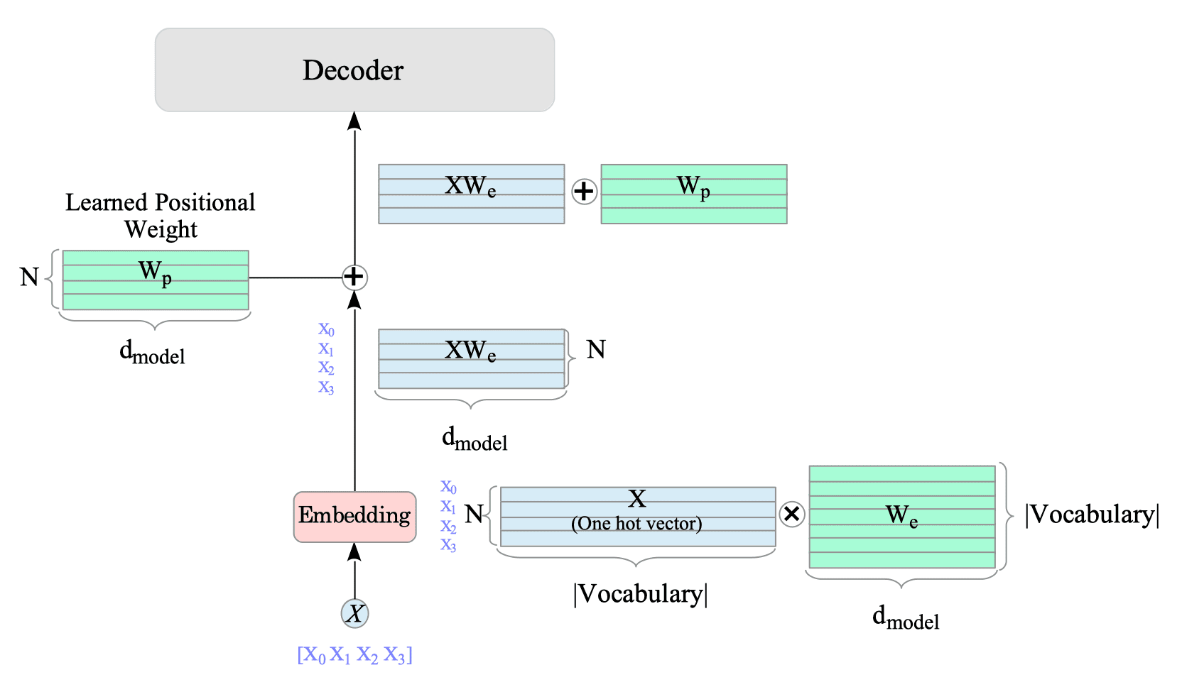
Fig.20-1: GPT-1's Positional Encoding Mechanism.
20.2.2. GPT-1 Model Formulation
This section formulates the forward computation of GPT-1 during the pre-training phase.
Figure 20.2 shows the GPT-1 model during the pre-training phase.
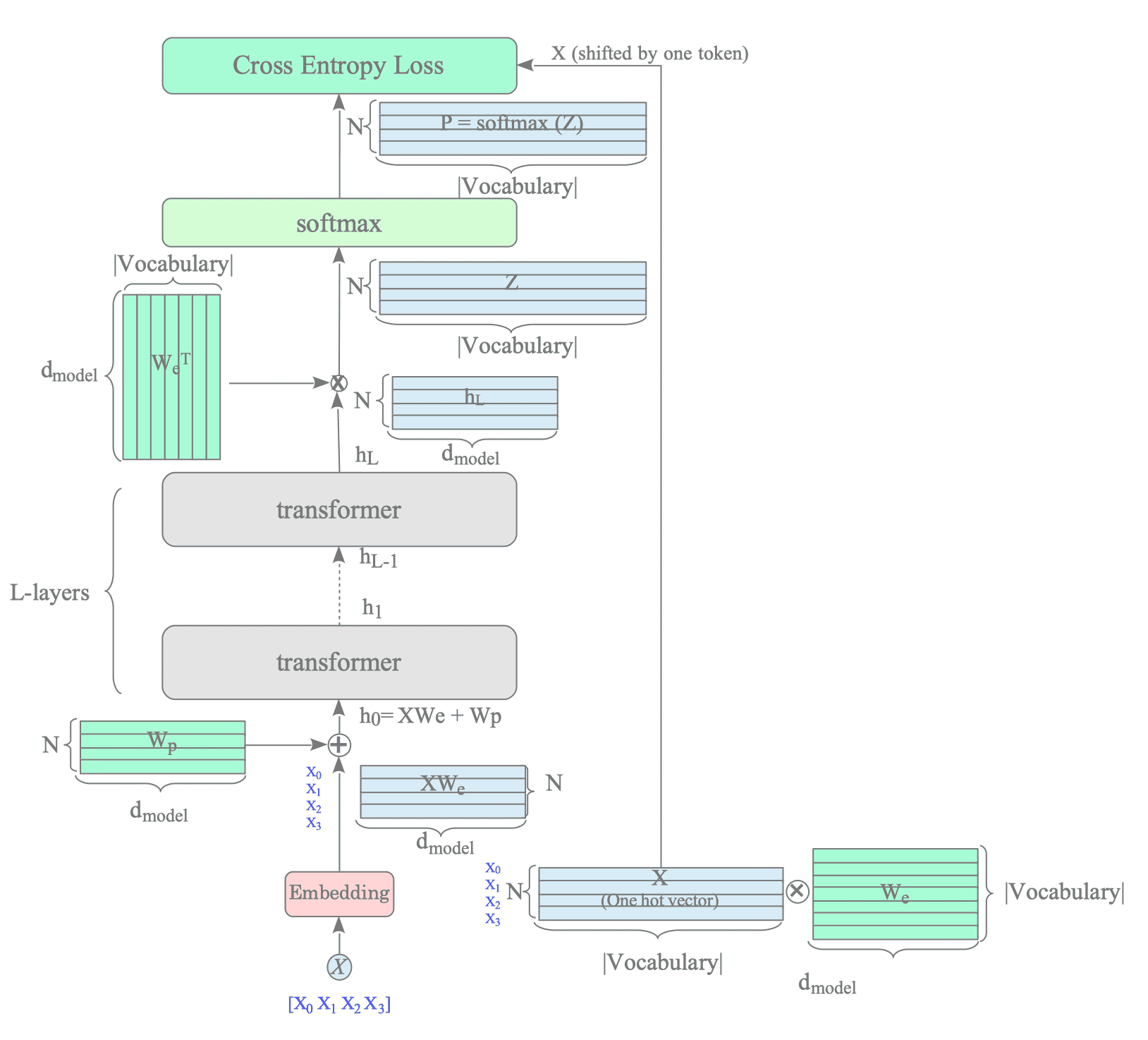
Fig.20-2: GPT-1 Pre-training Model.
To simplify the formal framework, let $h_{0}$ denote the combined input matrix $X_{pe}$ obtained from the token and position embeddings. Under this convention, the forward pass through the Transformer decoder blocks and the final output projection layer is defined as follows:
$$ \begin{cases} h_{0} = X W_{e} + W_{p} \\ h_{i} = \text{transformer_block}(h_{i-1}) \qquad \forall i \in [1, L] \\ Z = h_{L} W_{e}^{T} \\ P = \text{softmax}(Z) \end{cases} $$where:
- $Z \in \mathbb{R}^{N \times \vert{}\text{Vocabulary}\vert{}}$ is the matrix of logits produced by projecting the final decoder representations $h_{L}$ back onto the vocabulary space. (Note that GPT-1 ties the weights of the embedding and output projection layers by reusing $W_{e}^{T}$).
- $P \in \mathbb{R}^{N \times \vert{}\text{Vocabulary}\vert{}}$ is the matrix of predicted probability distributions over the vocabulary, obtained by applying the softmax function to each row of $Z$.
The $t$-th row of $P$ represents the predicted probability distribution for the next token, conditioned on the input tokens up to position $t$.
20.2.3. Loss Function
The pre-training objective is optimized using the cross-entropy loss.
The exact loss function $L_{p}$ using the input matrix $X$ (one-hot encoded) and the predicted probability matrix $P$ is expressed as follows:
$$ L_{p} = - \sum_{i=0}^{N-2} \sum_{j=0}^{|\text{Vocabulary}|-1} X_{i+1, j} \log(P_{i, j}) \tag{20-1} $$where:
- $N$ is the sequence length (number of rows).
- $\vert{}\text{Vocabulary}\vert{}$ represents the vocabulary size.
In a Causal Language Model (Causal LM), the ground truth target for the prediction at position $i$ ($P_i$) is the next token at position $i+1$ ($X_{i+1}$).
Since $X$ is composed of one-hot vectors, $X_{i}$ can be represented as follows, assuming the target word position is $k$:
$$X_{i} = \underbrace{ [0, \dots, 0, \overset{k\text{-th}}{1}, 0, \dots, 0] }_{\vert{}\text{Vocabulary}\vert{}}$$ $$X_{i,m} = \begin{cases} 1 \qquad k = m \\ 0 \qquad k \neq m \end{cases}$$For simplicity, let $y_{i}$ denote the position of the target word in $X_{i}$ (in the example above, $k = y_{i}$).
As a concrete example, consider the 4-token sequence [$X_{0}, X_{1}, X_{2}, X_{3}$] shown in Figure 20.2:
$$\begin{align} L_{p} &= - \sum_{j=0} X_{1, j} \log(P_{0, j}) - \sum_{j=0} X_{2, j} \log(P_{1, j}) - \sum_{j=0} X_{3, j} \log(P_{2, j}) \\ &= - \log(P_{0, y_{1}}) - \log(P_{1, y_{2}}) - \log(P_{2, y_{3}}) \\ &= - \sum_{i=0}^{2} \log(P_{i, y_{i+1}}) \end{align}$$Note that the final input token ($X_{3}$) does not contribute to the loss because there is no next token to predict.
Each term in the sum represents the cross-entropy loss at a specific step:
- First term: The loss between the prediction $P_{0}$ (from $X_{0}$) and the target token $X_{1}$.
- Second term: The loss between the prediction $P_{1}$ (from $X_{1}$) and the target token $X_{2}$.
- Third term: The loss between the prediction $P_{2}$ (from $X_{2}$) and the target token $X_{3}$.