2.2. Overview of Neural Network Training

To obtain the appropriate parameter values for neural networks, we can use optimization techniques. Here is an overview of how optimization techniques are used in neural networks:

1. Determine the loss function.
   The loss function, also known as the error function, measures the difference between the network’s output and the desired output (labels). A lower loss value indicates a closer match between the network’s prediction and the actual label.
   Common choices include:

   • Mean Squared Error (MSE): Used for regression tasks, where the network aims to predict continuous values.
   • Cross-Entropy Error (CE): Employed for classification tasks, where the network classifies inputs into discrete categories.

2. Use various (stochastic) gradient descent algorithms, which is explained in Appendix 2.3, to find the optimal parameters that minimize the loss value.

The second step is more complex, but it can be summarized as follows:

• Within each epoch (training iteration):
  1. Forward propagation: Compute the neural network’s output for a given input to obtain the loss value.
  2. Backpropagation: Compute the gradients of the neural network’s parameters.
  3. Parameter Update: Update weights and bias parameters using (stochastic) gradient descent algorithm.

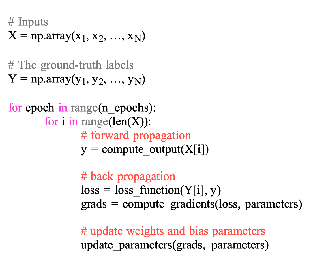
The training loop (the outer-loop) repeats until the loss reaches a minimum, indicating the network has learned.

As explained in Appendix 2.2.4, there are several ways to compute the derivative of a function, and modern frameworks like TensorFlow and PyTorch use automatic differentiation tools. The following Python code is an actual training function of XOR-gate model with Tensorflow.

model = SimpleNN(input_nodes, hidden_nodes, output_nodes)

loss_func = losses.MeanSquaredError()
optimizer = optimizers.Adam(learning_rate=0.1)

#
# Training function
#
@tf.function
def train(X, Y):
    with tf.GradientTape() as tape:
        # Forward Propagation
        y = model(X)

        # Back Propagation
        loss = loss_func(Y, y)
        grad = tape.gradient(loss, model.trainable_variables)

    # update weights and bias parameters
    optimizer.apply_gradients(zip(grad, model.trainable_variables))

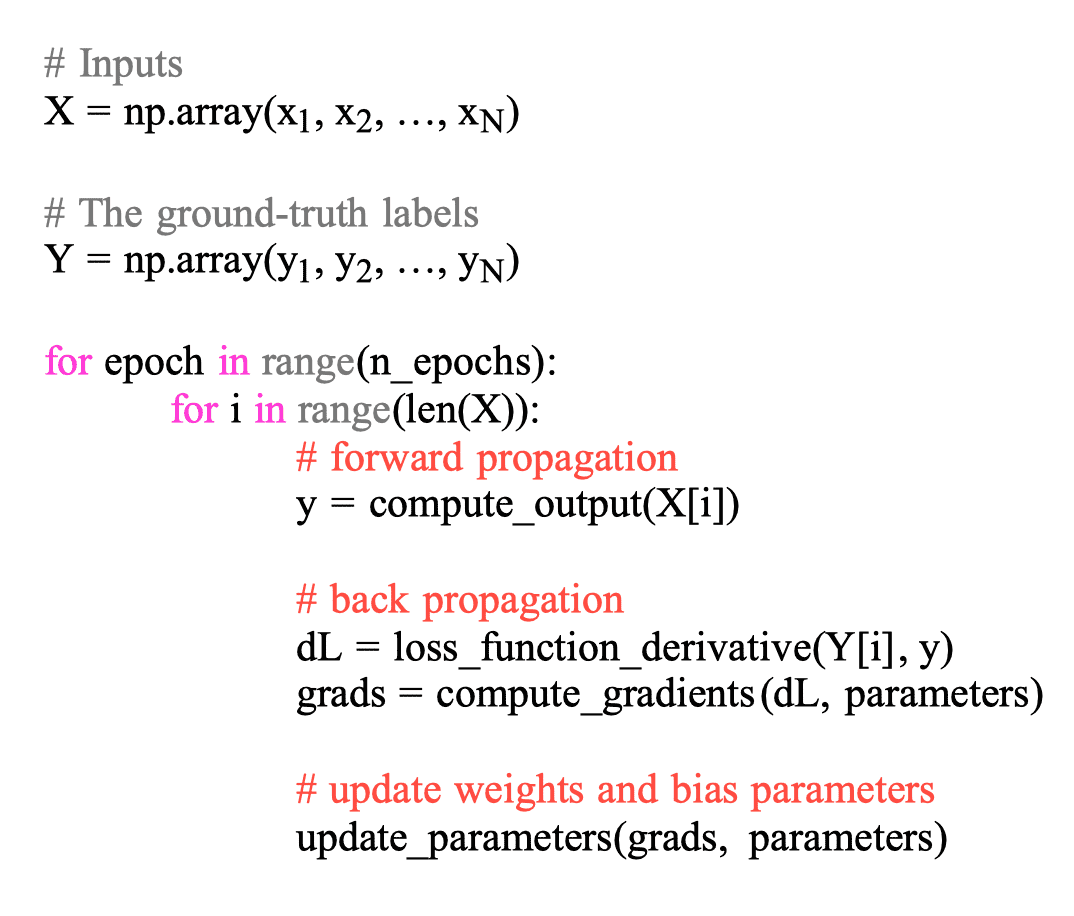
    return loss

In the examples of this chapter, however, we manually compute all gradients for better understanding of neural networks. Therefore, for the convenience of backpropagation calculations, we use the gradient value $\nabla L$ of the loss function, denoted by $dL$, instead of the loss function value $loss$.

In the next section, we will delve into the use of computational graphs to visualize and understand backpropagation. Following that, we will build a Python code for a neural network that solves the XOR-gate problem.