2.3. Computing Gradients for Back Propagation
To compute the gradients for back propagation in neural networks, we have to determine the loss function first. In this chapter, we will use the mean squared error (MSE) as our loss function because we solve this task as a logistic regression problem1.
The MSE is defined as follows:
$$ L(x) = \frac{1}{2}(y(x) - Y(x))^{2} $$where $y$ is the output of the neural network for input $x$, and $Y$ is the label data (desired output) for input $x$.
In the following, we simplify the expression by omitting $x$:
$$ L = \frac{1}{2}(y - Y)^{2} $$Before computing the derivatives, we define the gradient, denoted by $dL$, from a loss function $L$, which can be any loss function:
$$ \begin{align} dL & \stackrel{\mathrm{def}}{=} \frac{\partial L}{\partial y} \\ &= \frac{\partial \frac{1}{2}(y - Y)^{2}}{\partial (y - Y)} \frac{\partial (y - Y)}{\partial y} \\ &= (y - Y) \end{align} $$In this document, “$d$” denotes the gradient (e.g., $dL, dW, dU, db, dc$), not the total derivative.
Next, we build the backward computational graph of the neural network to compute the derivatives. To achieve it, we compute the derivatives between all the nodes of the forward graph. Fig.2-2 illustrates the forward computational graph of the neural network.
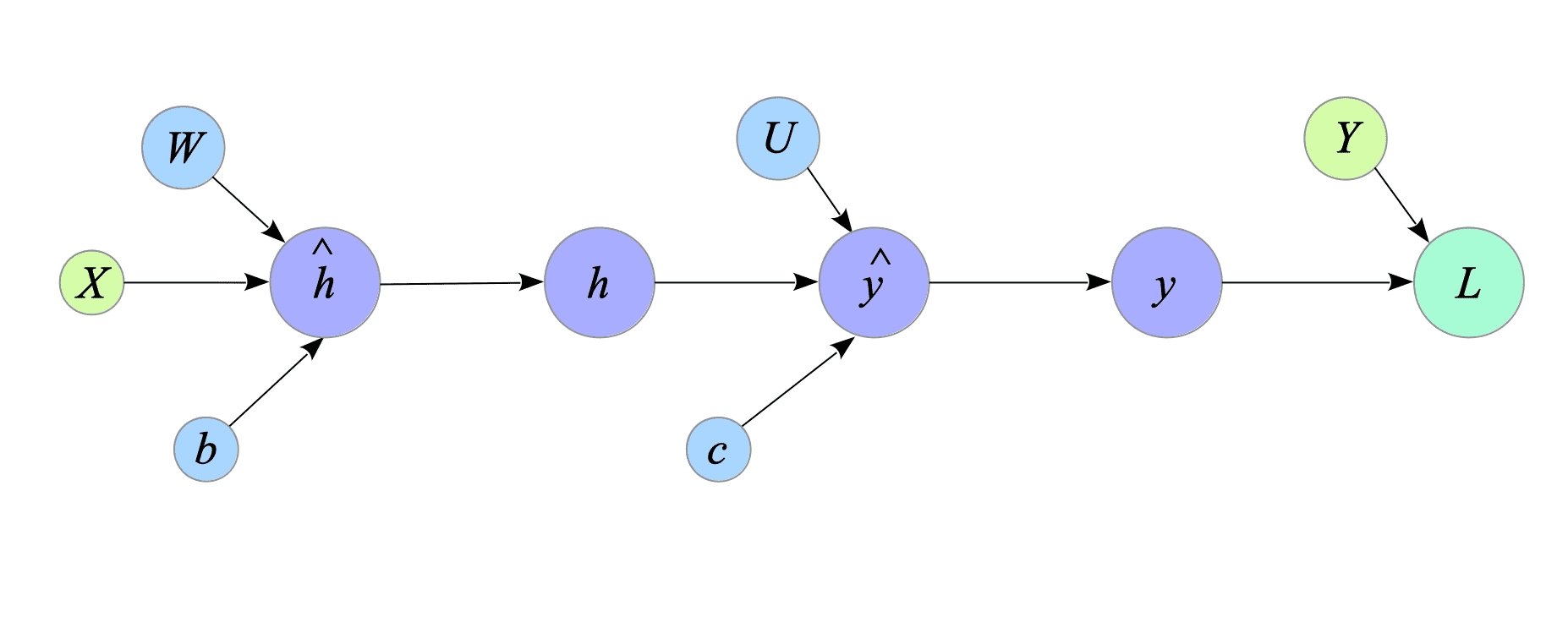
Fig.2-2: Forward Computational Graph of the Neural Network
For an explanation of computational graphs, see Appendix.
Using these computed derivatives, we can build the backward computational graph shown in Fig.2-3.
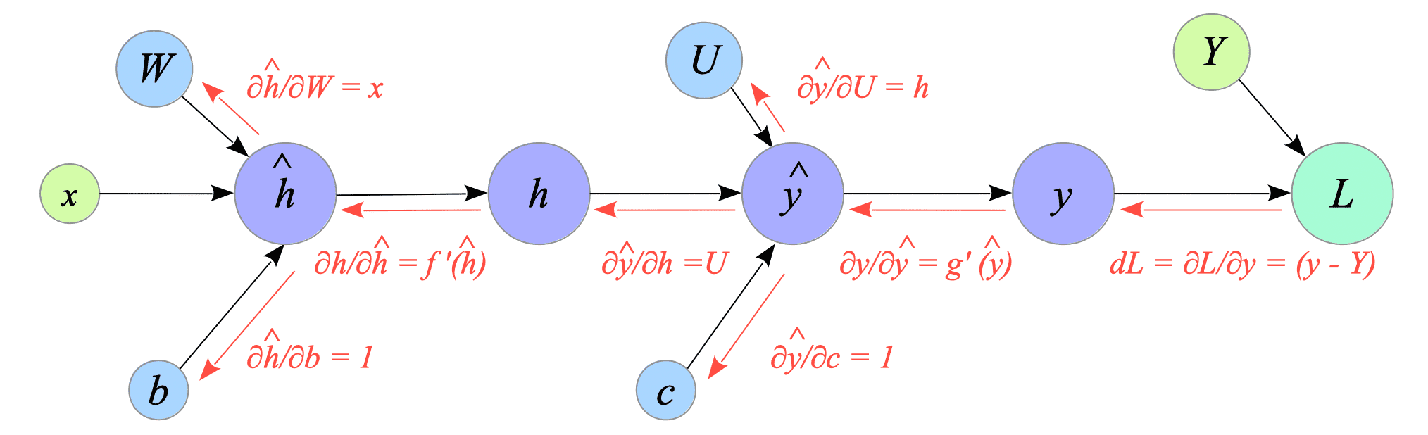
Fig.2-3: Backward Computational Graph of the Neural Network
Finally, we can obtain the gradients $\frac{\partial L}{\partial b}$, $\frac{\partial L}{\partial W}$, $\frac{\partial L}{\partial c}$ and $\frac{\partial L}{\partial U}$ (denoted by $db, dW, dc, dU$), using the backward computational graph shown above:
$$ \begin{align} db &\stackrel{\mathrm{def}}{=} \frac{\partial L}{\partial b} = \frac{\partial L}{\partial y} \frac{\partial y}{\partial \hat{y}} \frac{\partial \hat{y}}{\partial h} \frac{\partial h}{\partial \hat{h}} \frac{\partial \hat{h}}{\partial b} \\ &= g'(\hat{y}) U f'(\hat{h}) dL \\ dW &\stackrel{\mathrm{def}}{=} \frac{\partial L}{\partial W} = \frac{\partial L}{\partial y} \frac{\partial y}{\partial \hat{y}} \frac{\partial \hat{y}}{\partial h} \frac{\partial h}{\partial \hat{h}} \frac{\partial \hat{h}}{\partial W} \\ &= g'(\hat{y}) U f'(\hat{h}) x^{T} dL \\ &= db \ x^{T} \\ dc &\stackrel{\mathrm{def}}{=} \frac{\partial L}{\partial c} = \frac{\partial L}{\partial y} \frac{\partial y}{\partial \hat{y}} \frac{\partial \hat{y}}{\partial c} \\ &= g'(\hat{y}) dL \\ dU &\stackrel{\mathrm{def}}{=} \frac{\partial L}{\partial U} = \frac{\partial L}{\partial y} \frac{\partial y}{\partial \hat{y}} \frac{\partial \hat{y}}{\partial U} \\ &= g'(\hat{y}) h^{T} dL \\ &= dc \ h^{T} \end{align} $$-
Logistic regression is a statistical method used for binary classification problems, where the goal is to predict the probability that an instance belongs to a particular class. ↩︎