9.1. Formulation of GRU
The formulation of the GRU is defined as follows:
$$ \begin{cases} z^{(t)} = \sigma(W_{z} x^{(t)} + U_{z} h^{(t-1)} + b_{z}) \\ r^{(t)} = \sigma(W_{r} x^{(t)} + U_{r} h^{(t-1)} + b_{r}) \\ \hat{h}^{(t)} = \tanh(W x^{(t)} + ( r^{(t)} \odot h^{(t-1)}) U + b) \\ h^{(t)} = (1 - z^{(t)}) \odot h^{(t-1)} + z^{(t)} \odot \hat{h}^{(t)} \end{cases} \tag{9.1} $$Given that the number of input nodes and hidden nodes are $ m $ and $ h $, respectively, then:
- $ x^{(t)} \in \mathbb{R}^{m} $ is the input at time $t$.
- $ h^{(t)} \in \mathbb{R}^{h} $ is the hidden states at time $t$.
- $ W_{r}, W_{z} \in \mathbb{R}^{h \times m} $ are the weight matrices for the reset gate, update gate, respectively.
- $ U_{r}, U_{z} \in \mathbb{R}^{h \times h} $ are the recurrent weight matrices for the reset gate, update gate, respectively.
- $ b_{r}, b_{z} \in \mathbb{R}^{h} $ are the bias vectors for the reset gate, update gate, respectively.
- $ W \in \mathbb{R}^{h \times m} $ is the weight matrix, and $ U \in \mathbb{R}^{h \times h} $ is the recurrent weight matrix.
Fig.9-2 illustrates the GRU defined above:
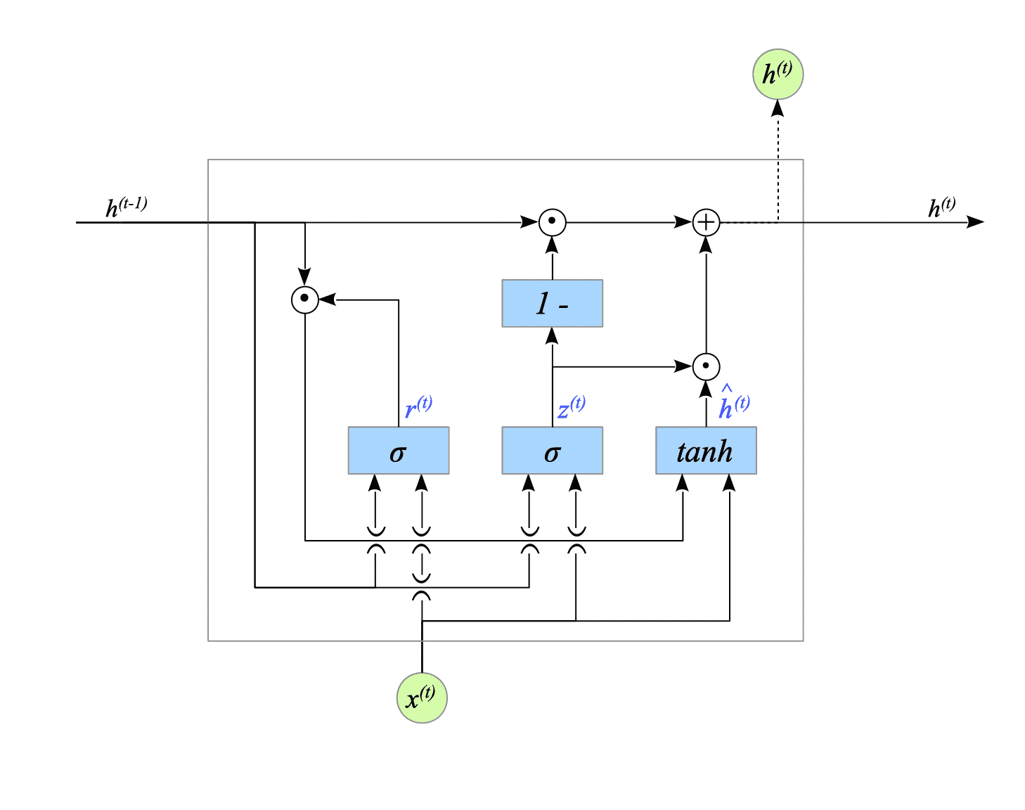
Fig.9-2: GRU unit
We add a dense layer to extract the final hidden state. This makes it a many-to-one GRU. See Fig.9-3.
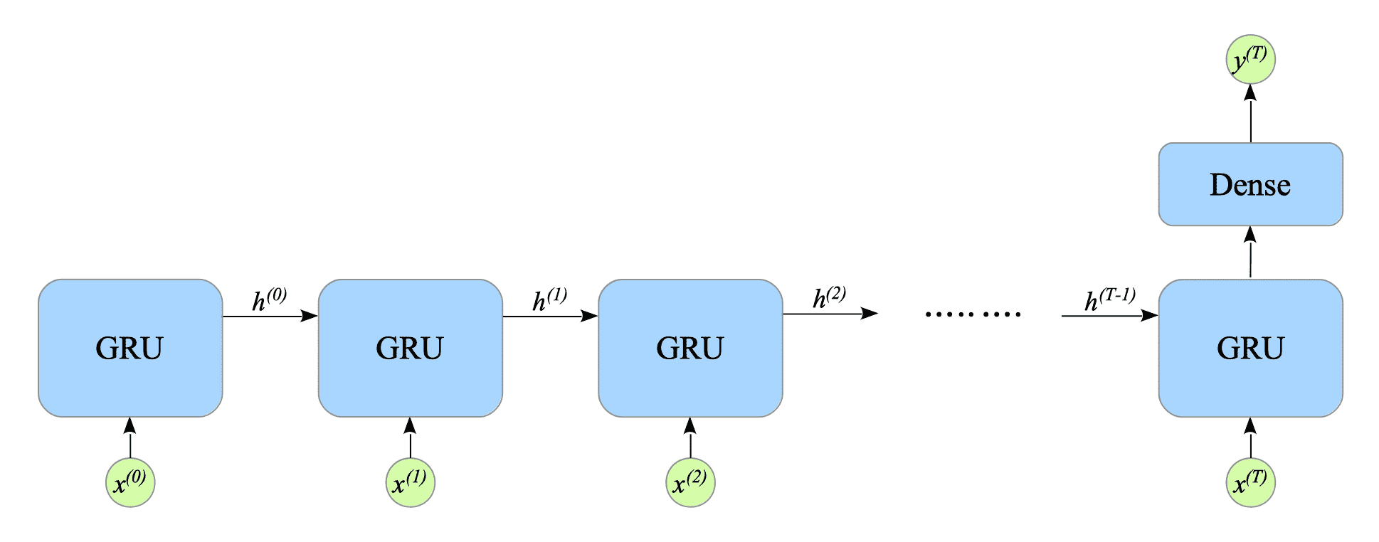
Fig.9-3: Many-to-One GRU
Given that the number of output nodes is $ n $. Then, the dense layer is defined as follows:
$$ y^{(T)} = g(V h^{(T)} + c) \tag{9.2} $$where:
- $ V \in \mathbb{R}^{n \times h} $ is the weight matrix.
- $ c \in \mathbb{R}^{n} $ is the bias term.
- $ y^{(T)} \in \mathbb{R}^{n} $ is the output vector.
- $ g(\cdot) $ is the activation function.