15.2. Multi-Head Attention
The Transformer model leverages three types of attention mechanisms:
-
Multi-Head (source-target) Attention:
The source-target attention mechanism connects the encoder and decoder. It is essentially the same as the attention mechanism in RNN-based translation models, but parallelized using multi-head attention. -
Multi-Head Self-Attention:
The self-attention, popularized by the Transformer model, focuses on learning the relationships between words within the input sequence. -
Masked Multi-Head Self-Attention:
The masked attention is applied to the decoder units to address the problem caused by processing the entire sequence simultaneously.
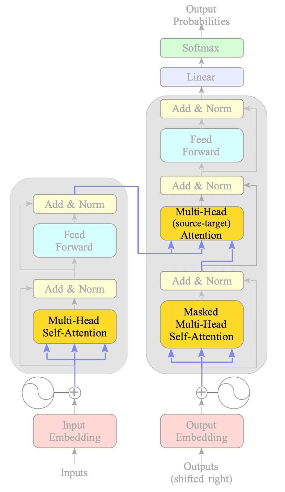
Fig.15-6: Three Types of Attention in the Transformer Model
The following sections will provide detailed explanations of each attention mechanism.
15.2.1. Multi-Head Attention
The multi-head attention mechanism can be mathematically expressed as follows:
$$ \text{MultiHead}(Q,K,V) = \text{Concat}(\text{head}_{1}, \ldots , \text{head}_{h}) W^{O} \tag{15.1} $$where $\text{head}_{i}$ is a scaled dot-product attention defined as follows:
$$ \begin{align} \text{head}_{i} &= \text{Attention}(Q W^{Q}_{i}, \ K W^{K}_{i}, \ V W^{V}_{i}) \\ &= \text{softmax} \left( \frac{ (Q W^{Q}_{i}) \ (K W^{K}_{i})^{T} }{\sqrt{d_{k}}} \right) (V W^{V}_{i}) \end{align} \tag{15.2} $$Fig.15-7 illustrates a multi-head attention and a scaled dot-product attention:
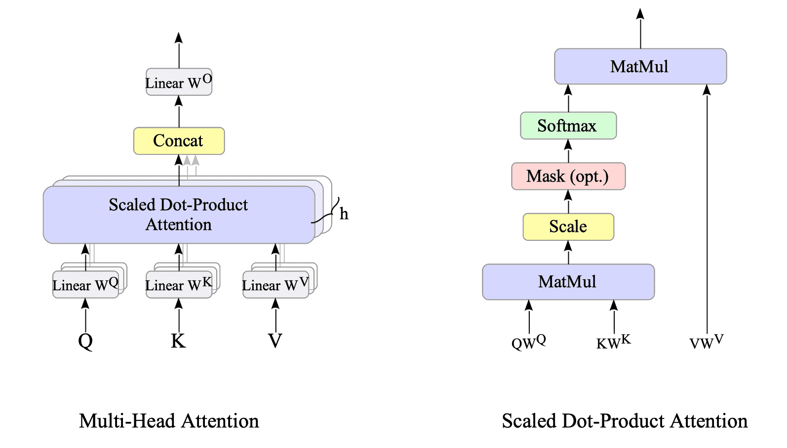
Fig.15-7: (Left) Multi-Head Attention Mechanism. (Right) Scaled Dot-Product Attention
We will delve into the matrix operations behind this mechanism.
$ Q, K, V \in \mathbb{R}^{N \times d_{model}} $ are input matrices, where $N$ is the length of input sentence, and $d_{model}$ is the word embedding dimension.
The $Q, K$, and $V$ matrices are multiplied by the $W^{Q}, W^{K}$, and $W^{V} \in \mathbb{R}^{d_{model} \times d_{model}} $ matrices by linear layers, respectively.
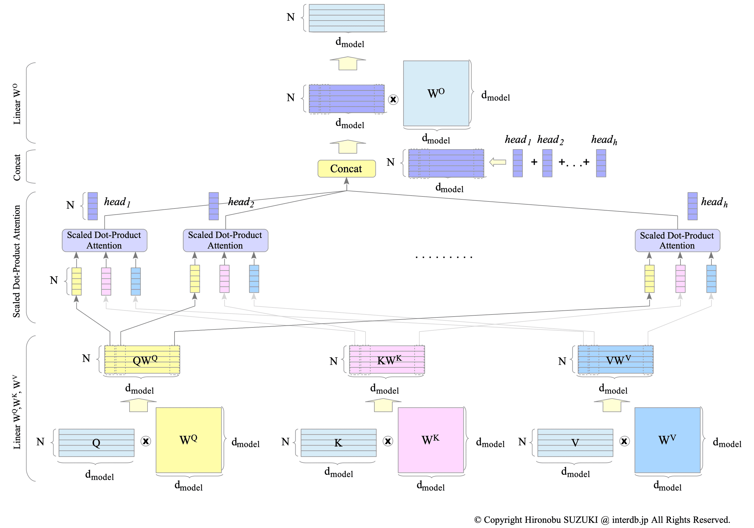
Fig.15-8: Multi-Head Attention
The multiplied matrices $QW^{Q}, KW^{K}$ and $VW^{V} \in \mathbb{R}^{N \times d_{model}}$ are split into $h$ heads as $Q W_{i}^{Q}, K W_{i}^{K} $ and $V W_{i}^{V} \in \mathbb{R}^{N \times \frac{d_{model}}{h}} $, and each portion of the matrices is provided to each scaled dot-product attention layer.
To simplify the expression, we introduce the following notation:
$$ d_{k} \stackrel{\mathrm{def}}{=} \frac{d_{model}}{h} $$According to the original paper, the reason why multi-head attention is utilized is its performance advantage:
Instead of performing a single attention function with $d_{model}$-dimensional keys, values and queries, we found it beneficial to linearly project the queries, keys and values $h$ times with different, learned linear projections to $d_{k}$, $d_{k}$ and $d_{v}$ dimensions, respectively.
Note that in the original paper, the expression $d_{v} = d_{h}$ is given.
- My understanding:
Multi-Head Attention (MHA) shares a resemblance to Convolutional Neural Networks (CNNs) in their ability to extract features from input data.
CNNs extract spatial features from images using multiple filters (kernels). Similarly, MHA employs multiple attention heads to capture different relationships within the input sequence. This effectively increases the model’s capacity to extract diverse and informative features from the sequence compared to a single-head model.
Each head, a scaled dot-product attention layer, returns a matrix $ head_{i} \in \mathbb{R}^{N \times d_{k}}$. These outputs are then concatenated to form the final result.
The original paper explains the reason for dividing dot products by $\sqrt{d_{k}}$ as follows:
We suspect that for large values of $d_{k}$, the dot products grow large in magnitude, pushing the softmax function into regions where it has extremely small gradients. To counteract this effect, we scale the dot products by $\frac{1}{\sqrt{d_{k}}}$.
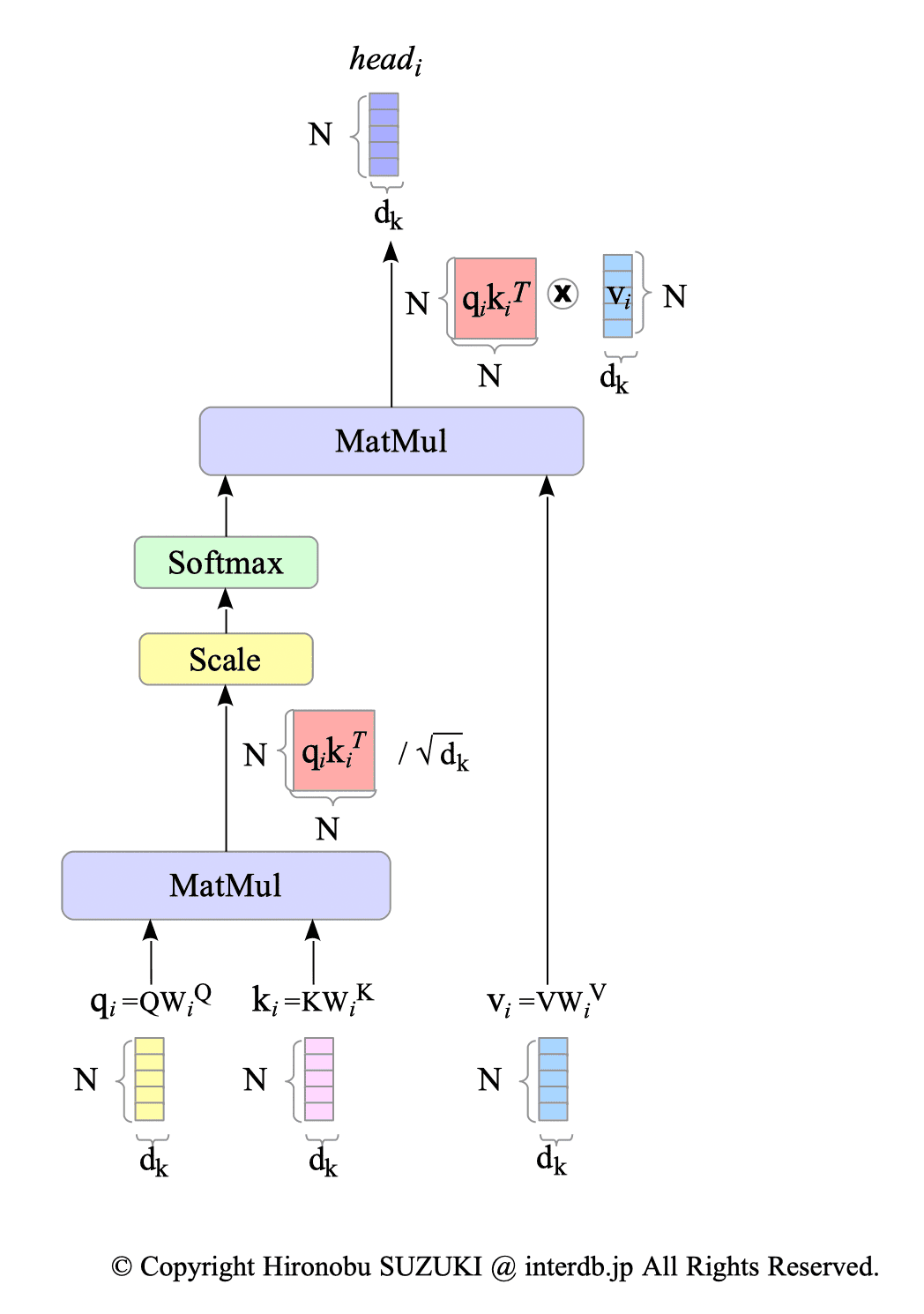
Fig.15-9: Scaled Dot-Product Attention
Finally, as shown by expression $(15.1)$, the concatenated head $ \text{Concat} (head_{1}, \ldots , head_{h}) $ is multiplied by the matrix $ W^{O} \in \mathbb{R}^{d_{model} \times d_{model}} $.
The scaled dot-product attention layer itself does not contain learnable weights or biases. This contributes to its computational efficiency, especially for long sequences.
Instead, the similarities among matrices $Q, K$, and $V$ are learned through the learnable weights of the linear layers preceding them: $W^{Q}$, $W^{K}$, and $W^{V}$.
15.2.1.1. Limitations and Complexity of Multi-Head Attention
The Transformer model has a maximum token length limitation, as mentioned in Section 15.1. This limitation is caused by computing the Scaled Dot-Product Attention on all tokens at the same time. In simpler terms, the model needs to pre-allocate fixed-size matrices, which requires setting a maximum token length.
Furthermore, this computation is computationally expensive, with a complexity of $\mathcal{O}(N^{2} \cdot d_{model} + N \cdot d_{model}^{2})$. Notably, when $N \gt d_{model}$, the complexity simplifies to $\mathcal{O}(N^{2} \cdot d_{model})$.
The complexity of the matrix multiplication $AB$, where $A \in \mathbb{R}^{l \times m} $ and $B \in \mathbb{R}^{m \times n} $, is $\mathcal{O}(l \cdot m \cdot n)$.
Therefore, the complexity of $q_{i} k_{i}^{T}$, where $q_{i}, k_{i} \in \mathbb{R}^{N \times d_{k}} $, is $\mathcal{O}(N^{2} \cdot d_{k})$. Similarly, the complexity of $ \text{softmax}(q_{i} k_{i}^{T}) v_{i} $, where $(q_{i} k_{i}^{T}) \in \mathbb{R}^{N \times N}$ and $v_{i} \in \mathbb{R}^{N \times d_{k}}$, is $\mathcal{O}(N^{2} \cdot d_{k})$.
Since $d_{k} = \frac{d_{model}}{h} $ by definition, and both $q_{i} k_{i}^{T}$ and $ (q_{i} k_{i}^{T}) v_{i} $ are computed in each head, the final complexity of scaled dot-product attention in Multi-head Attention is $\mathcal{O}(N^{2} \cdot \frac{d_{model}}{h} \cdot h) \Rightarrow \mathcal{O}(N^{2} \cdot d_{model})$.
The complexity of the multiplication between the concatenated outputs of scaled dot-product attention and the output projection matrix $W^{O} \in \mathbb{R}^{d_{model} \times d_{model}}$ is $\mathcal{O}(N \cdot d_{model}^{2})$.
Therefore, the overall complexity of Multi-Head Attention is $\mathcal{O}(N^{2} \cdot d_{model} + N \cdot d_{model}^{2})$.
Note that this complexity impacts not only computation time but also memory consumption significantly.
Section 17.1 will explore how researchers are addressing these bottlenecks.
15.2.1.2. Implementation
Here is a function for scaled dot-product attention and a class implementation of multi-head attention:
#
# Scaled dot product attention
#
def scaled_dot_product_attention(q, k, v, mask):
    matmul_qk = tf.matmul(q, k, transpose_b=True)
    dk = tf.cast(tf.shape(k)[-1], tf.float32)
    scaled_attention_logits = matmul_qk / tf.math.sqrt(dk)

    if mask is not None:
        scaled_attention_logits += mask * -1e9

    attention_weights = tf.nn.softmax(scaled_attention_logits, axis=-1)
    output = tf.matmul(attention_weights, v)

    return output, attention_weights

#
# Multi-head attention
#
class MultiHeadAttention(tf.keras.layers.Layer):
    def __init__(self, d_model, num_heads):
        super(MultiHeadAttention, self).__init__()
        self.num_heads = num_heads
        self.d_model = d_model

        assert d_model % self.num_heads == 0

        self.depth = d_model // self.num_heads

        self.Wq = tf.keras.layers.Dense(d_model)
        self.Wk = tf.keras.layers.Dense(d_model)
        self.Wv = tf.keras.layers.Dense(d_model)

        self.dense = tf.keras.layers.Dense(d_model)

    def call(self, v, k, q, mask):

        def _split_heads(x, batch_size):
            x = tf.reshape(x, (batch_size, -1, self.num_heads, self.depth))
            return tf.transpose(x, perm=[0, 2, 1, 3])


        batch_size = tf.shape(q)[0]

        q = self.Wq(q)
        k = self.Wk(k)
        v = self.Wv(v)

        q = _split_heads(q, batch_size)
        k = _split_heads(k, batch_size)
        v = _split_heads(v, batch_size)

        scaled_attention, attention_weights = scaled_dot_product_attention(q, k, v, mask)
        scaled_attention = tf.transpose(scaled_attention, perm=[0, 2, 1, 3])
        concat_attention = tf.reshape(scaled_attention, (batch_size, -1, self.d_model))
        output = self.dense(concat_attention)

        return output, attention_weights
15.2.2. Self-Attention
Similar to the RNN-based encoder-decoder model, the source-target attention mechanism in the Transformer model connects the encoder and decoder, establishing the relationship between the source language sentence and the target language sentence.
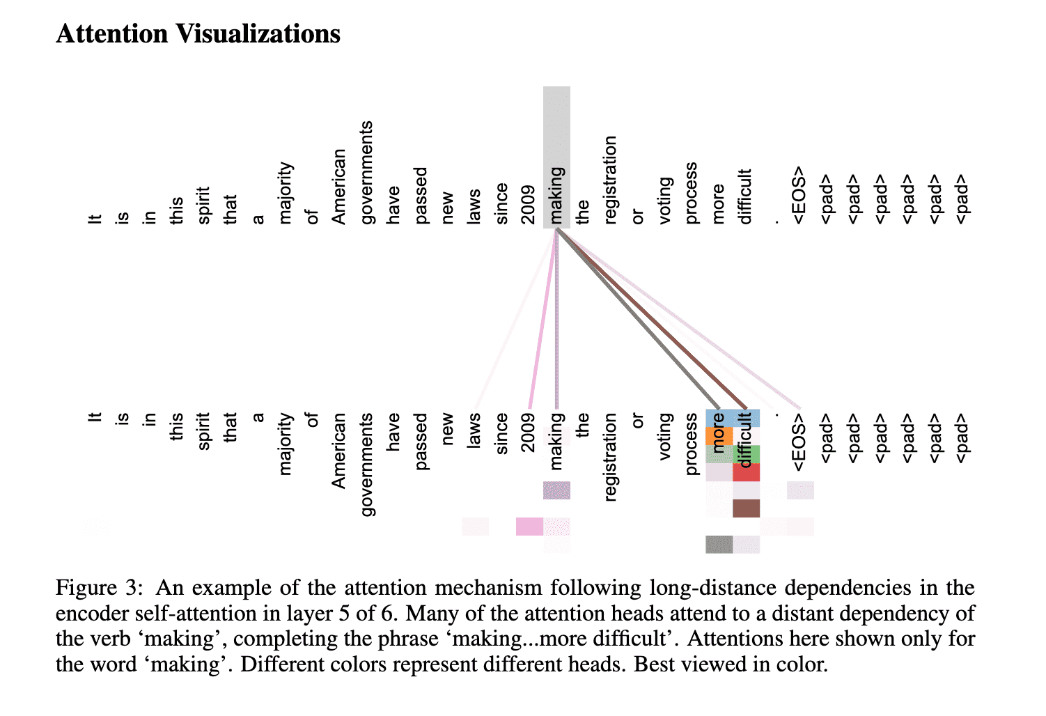
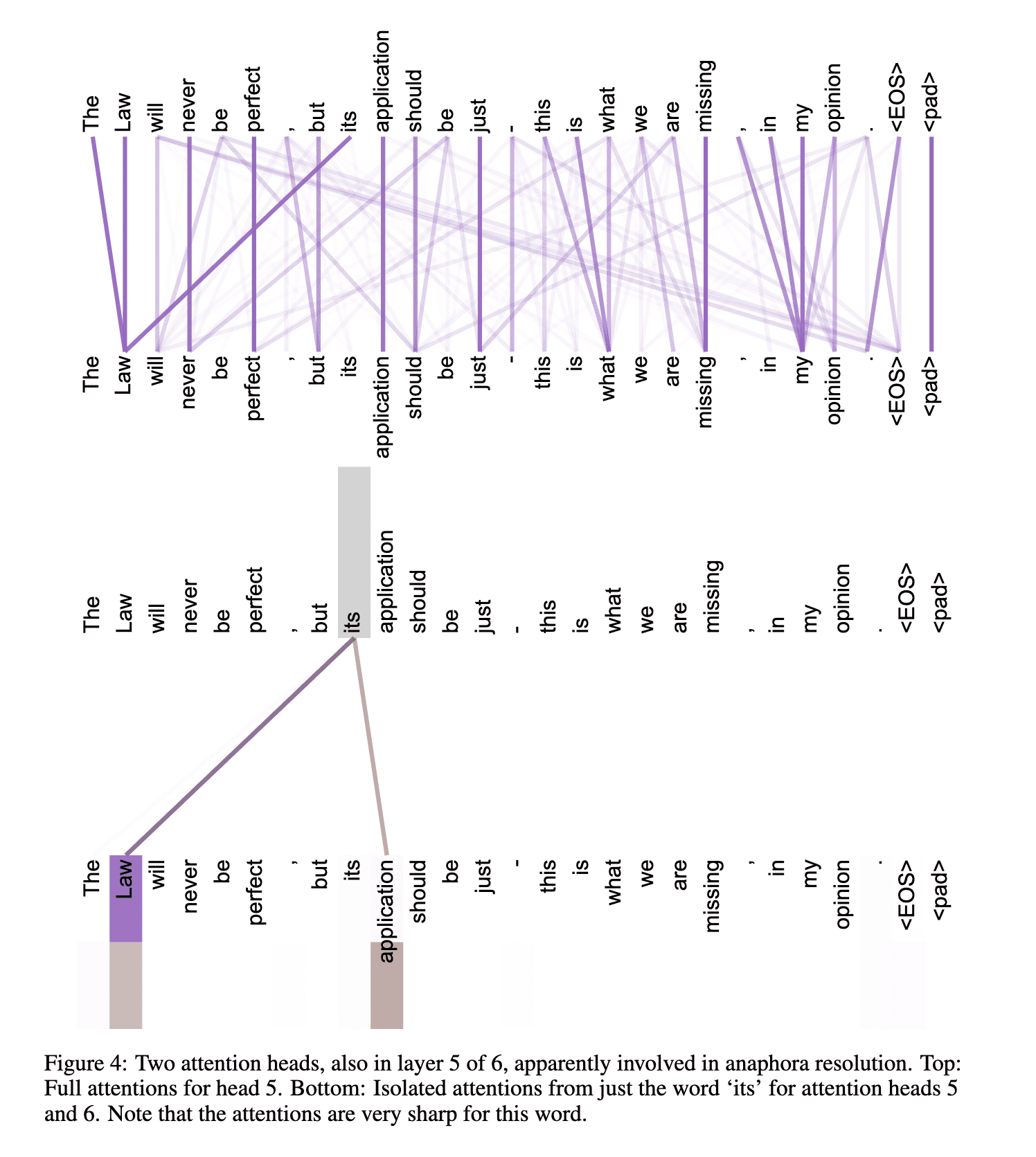
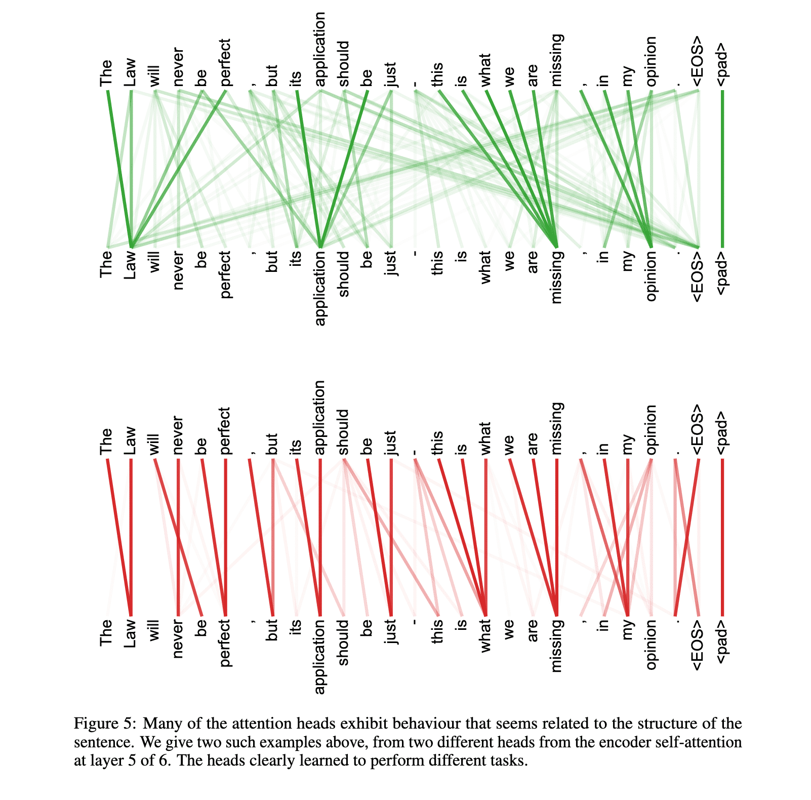
In contrast, the self-attention mechanism focuses on learning the relationships between words within the input sequence. This helps the model capture long-range dependencies within the sequence.
Interestingly, the authors of the Transformer paper modestly mention the influence of self-attention as follows:
As side benefit, self-attention could yield more interpretable models. We inspect attention distributions from our models and present and discuss examples in the appendix. Not only do individual attention heads clearly learn to perform different tasks, many appear to exhibit behavior related to the syntactic and semantic structure of the sentences.
Also see the Figures 3,4, and 5 of the original paper.
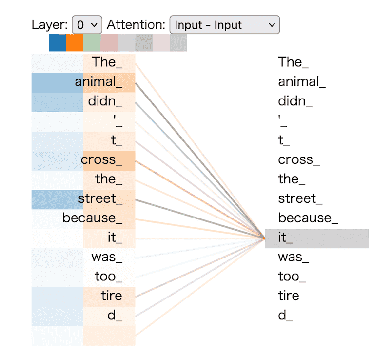
The following website provides an interactive feature that enables you to visualize the attention weights. I highly recommend to try it:
This is a screenshot of the website:
15.2.3. Masked Multi-Head Self-Attention
Unlike RNN-based machine translation models, the Transformer model fundamentally can process all tokens of a sentence simultaneously.
However, during translation, the Transformer’s decoder generates the output sequence one token at a time, similar to RNN-based models. To prevent the decoder from “cheating” by looking at future tokens, the Transformer employs masked self-attention.
Imagine you are studying for an exam. If you cheat by looking at the answers in advance, you would not learn how to perform well on the actual exam. Similarly, if the decoder were allowed to look at future tokens, it would not learn to generate the correct translation.
To prevent this cheating, the Transformer model uses a mask for scaled dot-product attention.
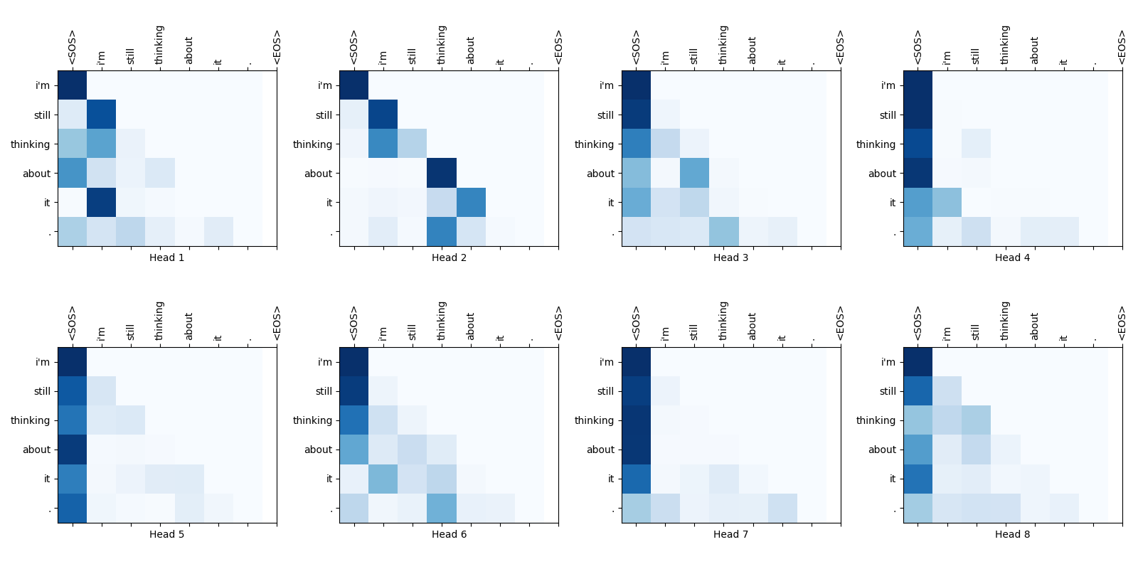
This mask hides future tokens in the sequence. As a result, the decoder is forced to rely on the information from past tokens and the current token itself when predicting the next word in the output sequence.
The following images provide an example of masked self-attention weight maps used in machine translation. The weights for future tokens are set to zero, indicating that the decoder is not allowed to refer to them.