12. Sequence Classification

In NLP, sequence classification models predict the category (label) a sequence of words belongs to. For example, in sentiment analysis, labels might be “positive” and “negative.”
Traditionally, Bayesian classifiers were used for sequence classification. However, modern approaches primarily leverage Transformer models like BERT.
While RNN-based methods haven’t been in popular, we will explore RNN-based sentiment analysis here. Its simplicity makes it a valuable exercise for understanding machine translation.
In this chapter, we will explore the following topics:
12.1. Definition
12.2. DataSet
12.3. Implementation
12.4. Sentiment Analysis
12.1. Definition of Sequence Classification
We have an input sequence $w_{1},\ldots,w_{n}$ with a corresponding label $l$ from a set of possible labels $L$. Estimating the label $l$ for the sequence $w_{1},\ldots,w_{n} $ can be expressed as:
$$ \hat{l} = \underset{l \in L}{argmax} \ P(l| w_{1:n}) $$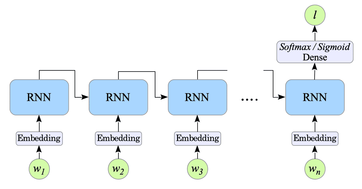
Fig.12-1: RNN-Based Sentiment Analysis
12.1.1. Intuitive Understanding of the Model
Here is an intuitive explanation of how the model predicts sentiment after sufficient training.
Consider the input sentence “It is good,” with a ground truth label of positive sentiment. During prediction, the model processes the sentence through the RNN, resulting in a final hidden state $h^{(n)}$. This hidden state captures the overall context of the sentence, thus it is called a context vector.
This context vector is then passed to a dense layer. This dense layer has already learned the relationship between context vectors and sentiment labels through training. Therefore, we expect the model to predict that the input sentence “It is good” reflects a positive sentiment.
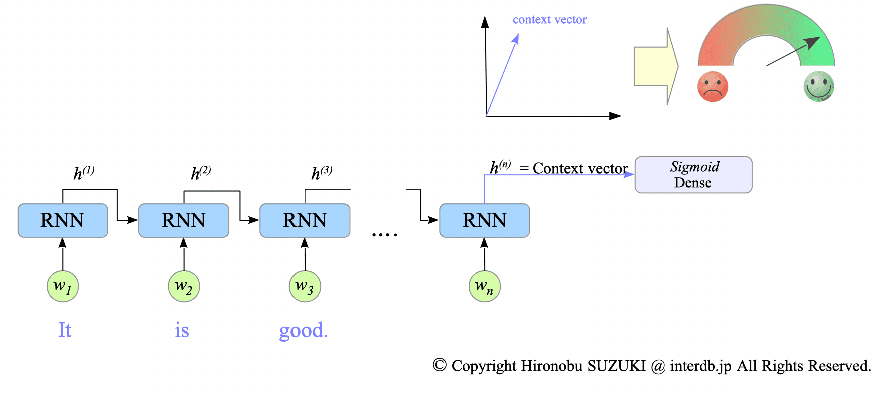
Fig.12-2: Processing the Input Sentence "It is good."
Conversely, when we feed the sentence “It is bad” (with a negative ground truth label), the model will returns different final hidden state due to the different sentence content. Consequently, the model will predict a negative label for this input.
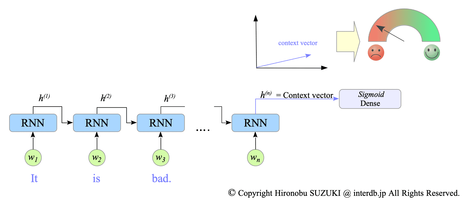
Fig.12-3: Processing the Input Sentence "It is bad."
12.2. DataSet
We will use the dataset:sentiment_labelled_sentences provided by The UCI Machine Learning Repository.
This repository provides three datasets1:
- amazon_cells_labelled.txt
- imdb_labelled.txt
- yelp_labelled.txt.
We specifically chose to work with the yelp_labelled.txt dataset. Here’s a sample of the first five lines:
$ head -5 ../DataSets/sentiment_labelled_sentences/yelp_labelled.txt
Wow... Loved this place.	1
Crust is not good.	0
Not tasty and the texture was just nasty.	0
Stopped by during the late May bank holiday off Rick Steve recommendation and loved it.	1
The selection on the menu was great and so were the prices.	1
Each line represents a sentence and its corresponding sentiment label.
A label of $1$ indicates a positive sentiment, while a $0$ represents negative sentiment.
Examples:
- the 1st line: “Wow… Loved this place.”, has a label of $1$, meaning it expresses a positive sentiment.
- the 2nd line: “Crust is not good.” has a label of $0$, meaning it expresses a negative sentiment.
12.3. Implementation
Complete Python code is available at: SentimentAnalysis-GRU-tf.py
12.3.1. Create Dataset
We create a dataset with input sequences represented as $X$ and corresponding labels as $Y$.
To ensure all input sequences have the same length ($\text{max_len}$), we pad shorter sequences with a special word, “<pad>”. This padding allows us to process sequences of varying lengths efficiently during batch processing.
input_text = "yelp_labelled.txt"

# ========================================
# Create dataset
# ========================================
split = True

file_path = "../DataSets/sentiment_labelled_sentences/" + input_text

Lang = li.LangIndex(file_path, category=True)
Lang.data_read(padding=True)

vocab_size = Lang.vocab_size()
max_len = Lang.max_len()

x = []
y = []

_pad = np.full(max_len, "<pad>")
_pad = np.array(_pad)


def padding(seq):
    w_len = len(seq)
    idxs = map(lambda w: Lang.word2idx[w], _pad[w_len:])
    for z in idxs:
        seq.append(z)
    return seq

for _, (sentence, label) in enumerate(zip(Lang.sentences, Lang.labels)):
    x.append(padding(sentence))
    y.append([label])

X = np.array(x)
Y = np.array(y)
Unlike previous examples, we use two separate datasets for training and validation. This allows us to train our model on the training data and evaluate its performance on the validation data, which the model hasn’t seen before. This separation ensures a fair evaluation of the model’s ability.
(X_train, X_validate, Y_train, Y_validate) = train_test_split(X, Y, test_size=0.2)

BUFFER_SIZE = int(X_train.shape[0])
BATCH_SIZE = 32
N_BATCH = BUFFER_SIZE // BATCH_SIZE

dataset = tf.data.Dataset.from_tensor_slices((X_train, Y_train)).shuffle(BUFFER_SIZE)
dataset = dataset.batch(BATCH_SIZE, drop_remainder=True)
12.3.2. Create Model
Our model comprises a word embedding layer, a many-to-one GRU network and a dense output layer.
-
Word Embedding Layer: The inputs passed through the word embedding layer before being fed into the GRU unit.
-
Many-to-one GRU Layer: We set $\text{return_sequences}=\text{False}$ and $\text{return_state}=\text{False}$ for the GRU network to achieve single output representation.
-
Dense Output Layer: As the labels are binary (positive or negative), we use the sigmoid activation function in the dense layer.
# ========================================
# Create Model
# ========================================

input_nodes = 1
hidden_nodes = 128
output_nodes = 1

embedding_dim = 64


class SentimentAnalysis(tf.keras.Model):
    def __init__(self, hidden_units, output_units, vocab_size, embedding_dim, rate=0.0):
        super().__init__()

        self.embedding = tf.keras.layers.Embedding(vocab_size, embedding_dim)

        self.gru = tf.keras.layers.GRU(
            hidden_units,
            activation="tanh",
            recurrent_activation="sigmoid",
            kernel_initializer="glorot_normal",
            recurrent_initializer="orthogonal",
            return_sequences=False,
            return_state=False,
        )
        self.dense = tf.keras.layers.Dense(output_units, activation="sigmoid")

    def call(self, x):
        x = self.embedding(x)
        context_vector = self.gru(x)
        x = self.dense(context_vector)
        return x


model = SentimentAnalysis(hidden_nodes, output_nodes, vocab_size, embedding_dim)

model.build(input_shape=(None, max_len))
model.summary()
12.4. Sentiment Analysis
The results of our RNN-based sentiment analysis on the validation dataset are presented below:
$ python SentimentAnalysis-GRU-tf.py
Model: "sentiment_analysis"
_________________________________________________________________
Layer (type) Output Shape Param #
=================================================================
embedding (Embedding) multiple 143808
gru (GRU) multiple 74496
dense (Dense) multiple 129
=================================================================
Total params: 218,433
Trainable params: 218,433
Non-trainable params: 0
... snip ...
Text:terrible management .
Correct value => Negative
Estimated value => Negative
Text:any grandmother can make a roasted chicken better than this one .
Correct value => Negative
Estimated value => Negative
Text:stopped by this place while in madison for the ironman very friendly kind staff .
Correct value => Positive
Estimated value => Positive
Text:it was extremely "crumby" and pretty tasteless .
Correct value => Negative
Estimated value => Negative
Text:the service was a bit lacking .
Correct value => Negative
Estimated value => Positive
*** Wrong ***
Text:their rotating beers on tap is also a highlight of this place .
Correct value => Positive
Estimated value => Negative
*** Wrong ***
Text:in an interesting part of town this place is amazing .
Correct value => Positive
Estimated value => Positive
Text:hell no will i go back .
Correct value => Negative
Estimated value => Negative
Text:and service was super friendly .
Correct value => Positive
Estimated value => Positive
Text:the staff are now not as friendly the wait times for being served are horrible no one even says hi for the first 10 minutes .
Correct value => Negative
Estimated value => Positive
*** Wrong ***
Text:total letdown i would much rather just go to the camelback flower shop and cartel coffee .
Correct value => Negative
Estimated value => Negative
Text:lobster bisque bussell sprouts risotto filet all needed salt and pepperand of course there is none at the tables .
Correct value => Negative
Estimated value => Negative
Text:the cashew cream sauce was bland and the vegetables were undercooked .
Correct value => Negative
Estimated value => Negative
Text:love this place hits the spot when i want something healthy but not lacking in quantity or flavor .
Correct value => Positive
Estimated value => Negative
*** Wrong ***
Text:i find wasting food to be despicable but this just wasnt food .
Correct value => Negative
Estimated value => Negative
Text:ive had better not only from dedicated boba tea spots but even from jenni pho .
Correct value => Negative
Estimated value => Negative
Text:very slow at seating even with reservation .
Correct value => Negative
Estimated value => Negative
Text:anyway this fs restaurant has a wonderful breakfast/lunch .
Correct value => Positive
Estimated value => Negative
*** Wrong ***
Text:i had the chicken pho and it tasted very bland .
Correct value => Negative
Estimated value => Positive
*** Wrong ***
Text:it was a pale color instead of nice and char and has no flavor .
Correct value => Negative
Estimated value => Negative
14 out of 20 sentences are correct.
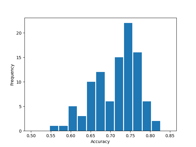
Accuracy: 0.720000In this example, 14 out of 20 sentences were correctly classified (sentence-level accuracy of 0.72).
After 100 trials, the average accuracy was 0.712 (standard deviation = 0.060).
-
The original dataset is available here: Sentiment Labelled Sentences. ↩︎