4.4. Exploding and Vanishing Gradients Problems
When many layers are stacked up, the gradients in neural networks can easily explode or vanish.
These problems are referred to exploding gradients problem and vanishing gradients problem.
To demonstrate the vanishing gradients problem, I created a Python program called XOR-gate-multi-hidden-layers.py. This program allows you to experiment with different numbers of hidden layers. Let’s try it and see what happens.
$ python XOR-gate-multi-hidden-layers.py
Input the number of residual connected hidden layers (1 to 10):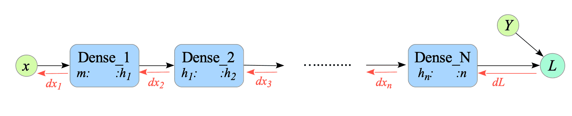
Fig.4-7: Pseudo-Computational Graph of XOR-Gate with Multiple Dense Layers
Enter the number of hidden layers you want, and then the program starts training.
$ python XOR-gate-multi-hidden-layers.py
Input the number of residual connected hidden layers (1 to 10): 10
_________________________________________________________________
 Layer (type)                Output Shape              Param #
=================================================================
 dense_in (Dense)            (None,  4)                   12
 dense_0 (Dense)             (None,  4)                   20
 dense_1 (Dense)             (None,  4)                   20
 dense_2 (Dense)             (None,  4)                   20
 dense_3 (Dense)             (None,  4)                   20
 dense_4 (Dense)             (None,  4)                   20
 dense_5 (Dense)             (None,  4)                   20
 dense_6 (Dense)             (None,  4)                   20
 dense_7 (Dense)             (None,  4)                   20
 dense_8 (Dense)             (None,  4)                   20
 dense_9 (Dense)             (None,  4)                   20
 dense_out (Dense)           (None,  1)                    5
=================================================================
Total params: 217

epoch: 1 / 100000  Loss = 0.732172
epoch: 1000 / 100000  Loss = 0.500135
epoch: 2000 / 100000  Loss = 0.500135
epoch: 3000 / 100000  Loss = 0.500135
epoch: 4000 / 100000  Loss = 0.500135
epoch: 5000 / 100000  Loss = 0.500134
epoch: 6000 / 100000  Loss = 0.500134
epoch: 7000 / 100000  Loss = 0.500134
epoch: 8000 / 100000  Loss = 0.500134

... snip ...

epoch: 97000 / 100000  Loss = 0.500124
epoch: 98000 / 100000  Loss = 0.500124
epoch: 99000 / 100000  Loss = 0.500124
epoch: 100000 / 100000  Loss = 0.500124

------------------------
x0 XOR x1 => result
========================
 0 XOR  0 => 0.5000
 0 XOR  1 => 0.5000
 1 XOR  0 => 0.5000
 1 XOR  1 => 0.5000
========================
In this program, setting 5 or more hidden layers either leads to vanishing gradients, preventing meaningful learning, or significantly increases the time needed for convergence to the desired result.
The following sections provide workarounds for these problems.
4.4.1. Exploding Gradients Problems
To prevent the gradient from exploding, gradients clipping can limit the magnitude of the gradients to a certain threshold. Its reference implementation is shown below:
def clip_gradient_norm(grads, max_norm=0.25):
    """
    g = (max_nrom/|g|)*g
    """
    max_norm = float(max_norm)
    total_norm = 0

    for grad in grads:
        grad_norm = np.sum(np.power(grad, 2))
        total_norm += grad_norm

    total_norm = np.sqrt(total_norm)
    clip_coef = max_norm / (total_norm + 1e-6)

    if clip_coef < 1:
        for grad in grads:
            grad *= clip_coef

    return grads
4.4.2. Vanishing Gradients Problems
To mitigate the vanishing gradient problem, various approaches have been developed:
- ReLU activation function
- Weight initialization
- Batch normalization
- Residual connections
Recurrent neural networks (RNNs) address the vanishing gradient problem using other approaches, which will be explained in Part 2.
4.4.2.1. ReLU activation function
Using the ReLU activation function is a countermeasure for the vanishing gradient problem, but it can also introduce the dying ReLU problem, which inhibits learning.
4.4.2.2. Weight Initialization
The weight Initialization is a technique of initializing the weights of the neural network in a way that prevents the gradient from vanishing. There are many different weight initialization techniques, such as Glorot initialization (a.k.a. Xavier initialization) and He initialization.
4.4.2.3. Batch Normalization
Batch normalization is a technique that normalizes the input to each layer of the neural network. This helps to alleviate the vanishing (and exploding) gradient problem.
4.4.2.4. Residual Connections
Residual connections1 are connections that skip one or more layers of the neural network. They help to prevent the gradient from vanishing by allowing the gradient to flow through the skipped layers.
Fig.4-8 illustrates the pseudo forward computational graphs of residual connections. The left connection skips one layer; the right connection skips two layers.
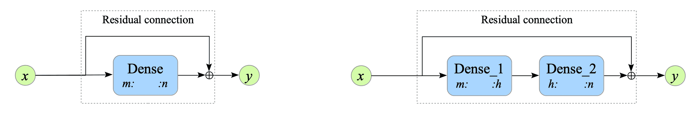
Fig.4-8: Pseudo-Forward Computational Graphs of Residual Connections
Fig.4-9 illustrates the pseudo backward computational graphs of residual connections.
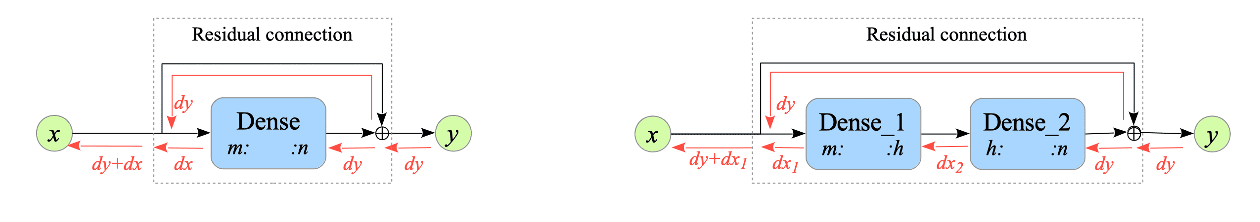
Fig.4-9: Pseudo-Backward Computational Graphs of Residual Connections
Here is the implementation of the residual class that skips one dense layer.
Complete Python code is available at: XOR-gate-residual-connection-layers.py
class ResidualConnection:
    def __init__(self, node_size, activate_func, deriv_activate_func):
        self.dense = Layers.Dense(node_size, node_size, activate_func, deriv_activate_func)

    def get_grads(self):
        return self.dense.get_grads()

    def get_params(self):
        return self.dense.get_params()

    def forward_prop(self, x):
        return x + self.dense.forward_prop(x)

    def back_prop(self, grads):
        return grads + self.dense.back_prop(grads)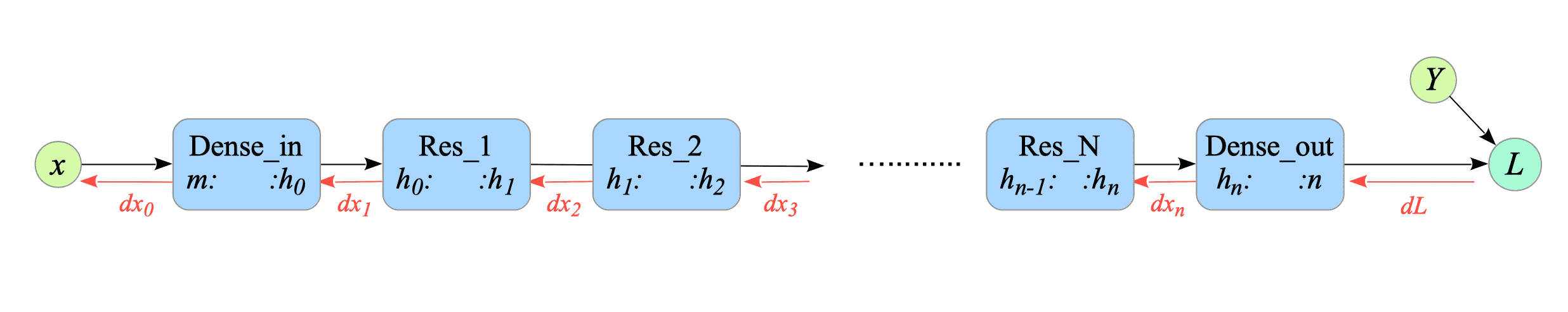
Fig.4-10: Pseudo-Computational Graph of XOR-Gate with Multiple Residual Connection Layers
Here is the result of running XOR-gate-residual-connection-layers.py:
$ python XOR-gate-residual-connection-layers.py
Input the number of hidden layers (1 to 10): 10
_________________________________________________________________
Layer (type)                Output Shape              Param #
=================================================================
 dense_in (Dense)            (None,  4)                   12
 residual_0 (Dense)          (None,  4)                   20
 residual_1 (Dense)          (None,  4)                   20
 residual_2 (Dense)          (None,  4)                   20
 residual_3 (Dense)          (None,  4)                   20
 residual_4 (Dense)          (None,  4)                   20
 residual_5 (Dense)          (None,  4)                   20
 residual_6 (Dense)          (None,  4)                   20
 residual_7 (Dense)          (None,  4)                   20
 residual_8 (Dense)          (None,  4)                   20
 residual_9 (Dense)          (None,  4)                   20
 dense_out (Dense)           (None,  1)                    5
=================================================================
Total params: 217

epoch: 1 / 100000  Loss = 1.000000
epoch: 1000 / 100000  Loss = 1.000000
epoch: 2000 / 100000  Loss = 1.000000
epoch: 3000 / 100000  Loss = 1.000000
epoch: 4000 / 100000  Loss = 0.499749
epoch: 5000 / 100000  Loss = 0.455718
epoch: 6000 / 100000  Loss = 0.358978
epoch: 7000 / 100000  Loss = 0.269385
epoch: 8000 / 100000  Loss = 0.032559
epoch: 9000 / 100000  Loss = 0.001467
epoch: 10000 / 100000  Loss = 0.000137
epoch: 11000 / 100000  Loss = 0.000016
epoch: 12000 / 100000  Loss = 0.000002
epoch: 13000 / 100000  Loss = 0.000000

------------------------
x0 XOR x1 => result
========================
 0 XOR  0 => 0.0001
 0 XOR  1 => 0.9998
 1 XOR  0 => 0.9998
 1 XOR  1 => 0.0004
========================
The results from XOR-gate-residual-connection-layers.py show that the network with 10 layers of residual connections successfully trained without the vanishing gradient. This suggests that residual connections effectively address this issue and potentially enable deeper architectures.
Although this is rare, convergence can be hindered by factors like initial values.
-
Residual connections were introduced by the ResNet architecture in the field of image recognition and are now a popular method used in deep learning. ↩︎