7.3. Implementation
Complete Python code is available at: RNN_from_scrtch.py
The simple RNN class is shown below:
class SimpleRNN:
    def __init__(self, input_units, hidden_units, activate_func, deriv_activate_func, return_sequences=False):
        self.input_units = input_units
        self.hidden_units = hidden_units

        self.activate_func = activate_func
        self.deriv_activate_func = deriv_activate_func

        self.return_sequences = return_sequences

        """
        Initialize random weights and bias using Glorot
        and Orthogonal Weight Initializations.

        Glorat Weight Initialization: Glorot & Bengio, AISTATS 2010
        http://jmlr.org/proceedings/papers/v9/glorot10a/glorot10a.pdf

        Orthogonal Weight Initialization: Saxe et al.,
        https://arxiv.org/pdf/1312.6120.pdf
        """
        self.W = np.random.randn(hidden_units, input_units) * np.sqrt(2.0 / (hidden_units + input_units))
        self.b = np.random.randn(hidden_units, 1) * np.sqrt(2.0 / (hidden_units + 1))
        self.U = np.random.randn(hidden_units, hidden_units) * np.sqrt(2.0 / (hidden_units + hidden_units))
        self.U, _, _ = np.linalg.svd(self.U) # Orthogonal Weight Initialization

    def get_grads(self):
        return [self.dW, self.dU, self.db]

    def get_params(self):
        return [self.W, self.U, self.b]

    def forward_prop(self, x, n_sequence):
        self.x = x
        self.n_sequence = n_sequence

        self.h = np.zeros([self.n_sequence, self.hidden_units, 1])
        self.h_h = np.zeros([self.n_sequence, self.hidden_units, 1])

        for t in range(self.n_sequence):
            self.h_h[t] = np.dot(self.W, x[t]) + self.b
            if t > 0:
                self.h_h[t] += np.dot(self.U, self.activate_func(self.h_h[t - 1]))
            self.h[t] = self.activate_func(self.h_h[t])

        if self.return_sequences == False:
            return self.h[-1]
        else:
            return self.h

    def back_prop(self, grads):

        dh = np.zeros([self.n_sequence, self.hidden_units, 1])
        dx = np.zeros([self.n_sequence, self.input_units, 1])

        # Compute dh from time step T backward through 0
        for t in reversed(range(self.n_sequence)):

            if t == self.n_sequence - 1:
                if self.return_sequences == True:
                    dh[t] = grads[t]
                else:
                    dh[t] = grads
            else:
                dh[t] = np.dot(self.U.T, dh[t + 1] * self.deriv_activate_func(self.h_h[t + 1]))
                if self.return_sequences == True:
                    dh[t] += grads[t]

        # Compute dW, db and dx from time step 0 through T
        for t in range(self.n_sequence):

            _db = dh[t] * self.deriv_activate_func(self.h_h[t])
            self.db += _db
            self.dW += np.dot(_db, self.x[t].T)
            if t > 0:
                self.dU += np.dot(_db, self.h[t - 1].T)

            dx[t] = np.dot(self.W.T, _db)

        return dx
The back_prop() method consists of two key steps:
-
Computing hidden state gradients: This loop iterates backward through time steps, starting from the final step $T$ and ending at $0$, to calculate the gradient of the hidden state at each step, denoted as $dh[t]$.
-
Calculating parameter gradients: Based on the computed hidden state gradients, this step calculates the gradients of the model’s parameters, including weights ($dW$), biases ($db$), and potentially input gradients ($dx$), with respect to the hidden state gradients.
[1] Create dataset.
n_sequence = 25
n_data = 100

n_sample = n_data - n_sequence  # number of samples

sin_data = ds.create_wave(n_data, 0.05)
X, Y = ds.dataset(sin_data, n_sequence)
[2] Create model.
We construct a simple RNN layer followed by a dense layer. The RNN utilizes a tanh activation function, while the dense layer employs a linear activation function.
input_units = 1
hidden_units = 32
output_units = 1

simple_rnn = SimpleRNN(input_units, hidden_units, tanh, deriv_tanh)
dense = Layers.Dense(hidden_units, output_units, linear, deriv_linear)
[3] Training.
This model’s training function is identical to the neural network training functions introduced so far.
def train(simple_rnn, dense, X, Y, optimizer):
    #
    # Forward Propagation
    #
    last_h = simple_rnn.forward_prop(X, n_sequence)
    y = dense.forward_prop(last_h)

    #
    # Back Propagation Through Time
    #
    loss = np.sum((y - Y) ** 2 / 2)
    dL = y - Y

    grads = dense.back_prop(dL)
    _ = simple_rnn.back_prop(grads)

    update_weights([dense, simple_rnn], optimizer=optimizer)

    return loss


history_loss = []

n_epochs = 200
lr = 0.0001

beta1 = 0.99
beta2 = 0.9999
optimizer = Optimizer.Adam(lr=lr, beta1=beta1, beta2=beta2)

for epoch in range(1, n_epochs + 1):

    loss = 0.0
    for j in range(n_sample):
        loss += train(simple_rnn, dense, X[j], Y[j], optimizer)
[4] Prediction.
Run the following command to generate and display the predicted sine wave:
$ python RNN_from_scratch.py
_________________________________________________________________
 Layer (type)                Output Shape              Param #
=================================================================
 simple_rnn (SimpleRNN)      (None,  25, 32)              1088
 dense (Dense)               (None,  25,  1)                33
=================================================================
Total params: 1121

epoch: 10/200	 Loss = 0.501159
epoch: 20/200	 Loss = 0.230240
epoch: 30/200	 Loss = 0.151318
epoch: 40/200	 Loss = 0.128992
epoch: 50/200	 Loss = 0.121157
epoch: 60/200	 Loss = 0.116868
epoch: 70/200	 Loss = 0.113596
epoch: 80/200	 Loss = 0.110712
epoch: 90/200	 Loss = 0.108037
epoch: 100/200	 Loss = 0.105510
epoch: 110/200	 Loss = 0.103115
epoch: 120/200	 Loss = 0.100848
epoch: 130/200	 Loss = 0.098704
epoch: 140/200	 Loss = 0.096684
epoch: 150/200	 Loss = 0.094783
epoch: 160/200	 Loss = 0.092997
epoch: 170/200	 Loss = 0.091322
epoch: 180/200	 Loss = 0.089752
epoch: 190/200	 Loss = 0.088284
epoch: 200/200	 Loss = 0.086911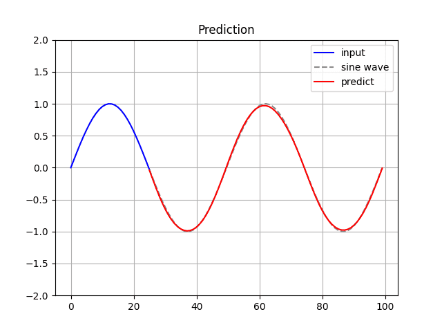
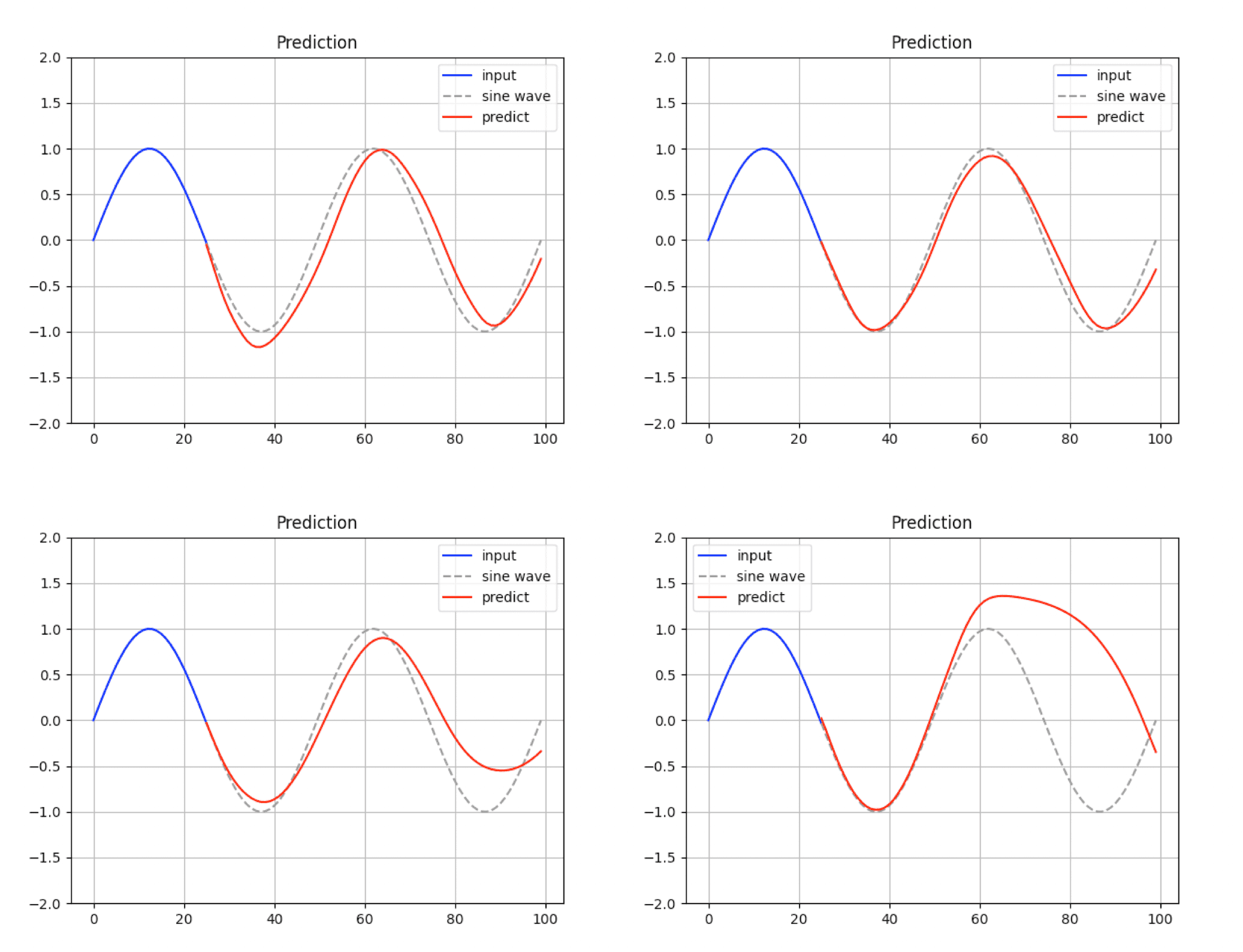
The model’s predictions can be inaccurate depending on the learned parameters.