8.3. Implementation
Complete Python code is available at: LSTM_from_scrtch.py
The LSTM class is shown below:
class LSTM:
    def __init__(self, input_units, hidden_units, return_sequences=False):
        self.return_sequences = return_sequences

        self.input_units = input_units
        self.hidden_units = hidden_units

        """
        Initialize random weights and bias using Glorot
        and Orthogonal Weight Initializations.

        Glorat Weight Initialization: Glorot & Bengio, AISTATS 2010
        http://jmlr.org/proceedings/papers/v9/glorot10a/glorot10a.pdf

        Orthogonal Weight Initialization: Saxe et al.,
        https://arxiv.org/pdf/1312.6120.pdf
        """
        self.Wi = np.random.randn(hidden_units, input_units) * np.sqrt(2.0 / (hidden_units + input_units))
        self.Wf = np.random.randn(hidden_units, input_units) * np.sqrt(2.0 / (hidden_units + input_units))
        self.Wc = np.random.randn(hidden_units, input_units) * np.sqrt(2.0 / (hidden_units + input_units))
        self.Wo = np.random.randn(hidden_units, input_units) * np.sqrt(2.0 / (hidden_units + input_units))

        self.Ui = np.random.randn(hidden_units, hidden_units) * np.sqrt(2.0 / (2 * hidden_units))
        self.Ui, _, _ = np.linalg.svd(self.Ui) # Orthogonal Weight Initialization
        self.Uf = np.random.randn(hidden_units, hidden_units) * np.sqrt(2.0 / (2 * hidden_units))
        self.Uf, _, _ = np.linalg.svd(self.Uf) # Orthogonal Weight Initialization
        self.Uc = np.random.randn(hidden_units, hidden_units) * np.sqrt(2.0 / (2 * hidden_units))
        self.Uc, _, _ = np.linalg.svd(self.Uc) # Orthogonal Weight Initialization
        self.Uo = np.random.randn(hidden_units, hidden_units) * np.sqrt(2.0 / (2 * hidden_units))
        self.Uo, _, _ = np.linalg.svd(self.Uo) # Orthogonal Weight Initialization

        self.bi = np.random.randn(hidden_units, 1) * np.sqrt(2.0 / (1 + hidden_units))
        self.bf = np.random.randn(hidden_units, 1) * np.sqrt(2.0 / (1 + hidden_units))
        self.bc = np.random.randn(hidden_units, 1) * np.sqrt(2.0 / (1 + hidden_units))
        self.bo = np.random.randn(hidden_units, 1) * np.sqrt(2.0 / (1 + hidden_units))


    def get_grads(self):
        return [self.dWi, self.dWf, self.dWc, self.dWo,
                self.dUi, self.dUf, self.dUc, self.dUo,
                self.dbi, self.dbf, self.dbc, self.dbo]

    def get_params(self):
        return [self.Wi, self.Wf, self.Wc, self.Wo,
                self.Ui, self.Uf, self.Uc, self.Uo,
                self.bi, self.bf, self.bc, self.bo]

    def forward_prop(self, x, n_sequence):
        self.x = x
        self.n_sequence = n_sequence

        self.h = np.zeros([self.n_sequence, self.hidden_units, 1])
        self.C = np.zeros([self.n_sequence, self.hidden_units, 1])

        self.i = np.zeros([self.n_sequence, self.hidden_units, 1])
        self.i_p = np.zeros([self.n_sequence, self.hidden_units, 1])
        self.c_h = np.zeros([self.n_sequence, self.hidden_units, 1])
        self.c_h_p = np.zeros([self.n_sequence, self.hidden_units, 1])
        self.f = np.zeros([self.n_sequence, self.hidden_units, 1])
        self.f_p = np.zeros([self.n_sequence, self.hidden_units, 1])
        self.o = np.zeros([self.n_sequence, self.hidden_units, 1])
        self.o_p = np.zeros([self.n_sequence, self.hidden_units, 1])

        for t in range(self.n_sequence):
            if t == 0:
                self.f_p[t] = np.dot(self.Wf, self.x[t]) + self.bf
                self.i_p[t] = np.dot(self.Wi, self.x[t]) + self.bi
                self.c_h_p[t] = np.dot(self.Wc, self.x[t]) + self.bc
                self.o_p[t] = np.dot(self.Wo, self.x[t]) + self.bo
            else:
                self.f_p[t] = (np.dot(self.Wf, self.x[t]) + np.dot(self.Uf, self.h[t - 1]) + self.bf)
                self.i_p[t] = (np.dot(self.Wi, self.x[t]) + np.dot(self.Ui, self.h[t - 1]) + self.bi)
                self.c_h_p[t] = (np.dot(self.Wc, self.x[t]) + np.dot(self.Uc, self.h[t - 1]) + self.bc)
                self.o_p[t] = (np.dot(self.Wo, self.x[t]) + np.dot(self.Uo, self.h[t - 1]) + self.bo)

            self.f[t] = sigmoid(self.f_p[t])
            self.i[t] = sigmoid(self.i_p[t])
            self.c_h[t] = tanh(self.c_h_p[t])
            self.o[t] = sigmoid(self.o_p[t])
            self.C[t] = (
                self.i[t] * self.c_h[t]
                if t == 0
                else self.i[t] * self.c_h[t] + self.f[t] * self.C[t - 1]
            )
            self.h[t] = self.o[t] * tanh(self.C[t])

        if self.return_sequences == False:
            return self.h[-1]
        else:
            return self.h

    def back_prop(self, grads):

        dh = np.zeros([self.n_sequence, self.hidden_units, 1])
        dC = np.zeros([self.n_sequence, self.hidden_units, 1])

        dx = np.zeros([self.n_sequence, self.input_units, 1])

        # Compute dh and dC from time step T backward through 0.
        for t in reversed(range(self.n_sequence)):

            if t == self.n_sequence - 1:
                if self.return_sequences == True:
                    dh[t] = grads[t]
                else:
                    dh[t] = grads

                dC[t] = dh[t] * self.o[t] * deriv_tanh(self.C[t])
            else:
                d1 = np.dot(self.Uo.T, dh[t + 1] * tanh(self.C[t + 1]) * deriv_sigmoid(self.o_p[t + 1]))
                d2 = np.dot(self.Ui.T, dh[t + 1] * self.o[t + 1] * deriv_tanh(self.C[t + 1]) * self.c_h[t + 1] * deriv_sigmoid(self.i_p[t + 1]))
                d3 = np.dot(self.Uc.T, dh[t + 1] * self.o[t + 1] * deriv_tanh(self.C[t + 1]) * self.i[t + 1] * deriv_tanh(self.c_h_p[t + 1]))
                d4 = np.dot(self.Uf.T, dh[t + 1] * self.o[t + 1] * deriv_tanh(self.C[t + 1]) * self.C[t] * deriv_sigmoid(self.f_p[t + 1]))

                dh[t] = d1 + d2 + d3 + d4
                if self.return_sequences == True:
                    dh[t] += grads[t]

                dC[t] = (dh[t] * self.o[t] * deriv_tanh(self.C[t]) + dC[t + 1] * self.f[t + 1])

        # Compute the gradients from time step 0 through T.
        for t in range(self.n_sequence):

            _do = dh[t] * tanh(self.C[t]) * deriv_sigmoid(self.o_p[t])
            self.dbo += _do
            self.dWo += np.dot(_do, self.x[t].T)
            if t > 0:
                self.dUo += np.dot(_do, self.h[t - 1].T)

            _di = dC[t] * self.c_h[t] * deriv_sigmoid(self.i_p[t])
            self.dbi += _di
            self.dWi += np.dot(_di, self.x[t].T)
            if t > 0:
                self.dUi += np.dot(_di, self.h[t - 1].T)

            _dc = dC[t] * self.i[t] * deriv_tanh(self.c_h_p[t])
            self.dbc += _dc
            self.dWc += np.dot(_dc, self.x[t].T)
            if t > 0:
                self.dUc += np.dot(_dc, self.h[t - 1].T)

            if t > 0:
                _df = dC[t] * self.C[t - 1] * deriv_sigmoid(self.f_p[t])
                self.dbf += _df
                self.dWf += np.dot(_df, self.x[t].T)
                self.dUf += np.dot(_df, self.h[t - 1].T)

            dx[t] = (np.dot(self.Wo.T, _do) + np.dot(self.Wi.T, _di) + np.dot(self.Wc.T, _dc))
            if t > 0:
                dx[t] += np.dot(self.Wf.T, _df)


        return dx
The back_prop() method consists of two key steps:
-
Computing hidden state gradients: This loop iterates backward through time steps, starting from the final step $T$ and ending at $0$, to calculate the gradients of the hidden and cell states at each step, denoted as $dh[t]$ and $dC[t]$.
-
Calculating parameter gradients: Based on the computed hidden state gradients, this step calculates the gradients of the model’s parameters, with respect to the hidden and cell states gradients.
[1] Create dataset.
# ============================
# Create Dataset
# ============================
n_sequence = 25
n_data = 100

n_sample = n_data - n_sequence  # number of samples

sin_data = ds.create_wave(n_data, 0.05)
X, Y = ds.dataset(sin_data, n_sequence)
[2] Create model.
We construct a LSTM layer followed by a dense layer. The dense layer employs a linear activation function.
# ============================
# Create Model
# ============================

input_units = 1
hidden_units = 32
output_units = 1

lstm = LSTM(input_units, hidden_units)
dense = Layers.Dense(hidden_units, output_units, linear, deriv_linear)
[3] Training.
This model’s training function is identical to the neural network training functions introduced so far
def train(lstm, dense, X, Y, optimizer):
# Forward Propagation
last_h = lstm.forward_prop(X, n_sequence)
y = dense.forward_prop(last_h)
# Back Propagation Through Time
loss = np.sum((y - Y) ** 2 / 2)
dL = y - Y
grads = dense.back_prop(dL)
_ = lstm.back_prop(grads)
update_weights([dense, lstm], optimizer=optimizer)
return loss
history_loss = []
n_epochs = 200
lr = 0.0001
beta1 = 0.99
beta2 = 0.9999
optimizer = Optimizer.Adam(lr=lr, beta1=beta1, beta2=beta2)
for epoch in range(1, n_epochs + 1):
loss = 0.0
for j in range(n_sample):
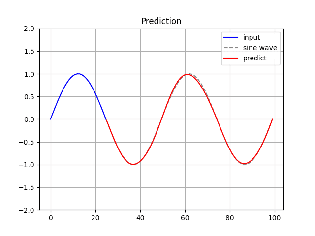
loss += train(lstm, dense, X[j], Y[j], optimizer)[4] Prediction.
Run the following command to generate and display the predicted sine wave:
$ python LSTM_from_scratch.py
_________________________________________________________________
 Layer (type)                Output Shape              Param #
=================================================================
 lstm (LSTM)                 (None,  25, 32)              4352

 dense (Dense)               (None,  25,  1)                33
=================================================================
Total params: 4385
epoch: 10/200	 Loss = 2.324861
epoch: 20/200	 Loss = 1.085645
epoch: 30/200	 Loss = 0.479348
epoch: 40/200	 Loss = 0.238478
epoch: 50/200	 Loss = 0.184795
epoch: 60/200	 Loss = 0.168116
epoch: 70/200	 Loss = 0.159275
epoch: 80/200	 Loss = 0.154013
epoch: 90/200	 Loss = 0.150791
epoch: 100/200	 Loss = 0.148719
epoch: 110/200	 Loss = 0.147262
epoch: 120/200	 Loss = 0.146123
epoch: 130/200	 Loss = 0.145147
epoch: 140/200	 Loss = 0.144262
epoch: 150/200	 Loss = 0.143434
epoch: 160/200	 Loss = 0.142646
epoch: 170/200	 Loss = 0.141890
epoch: 180/200	 Loss = 0.141164
epoch: 190/200	 Loss = 0.140462
epoch: 200/200	 Loss = 0.139785