4.1. Dense Layer (a.k.a. Fully Connected layer)
Referring back to Fig.2-2 in Section 2.3, the computational graph mainly consists of two elements: Dense layer, also known as Fully Connected layer.
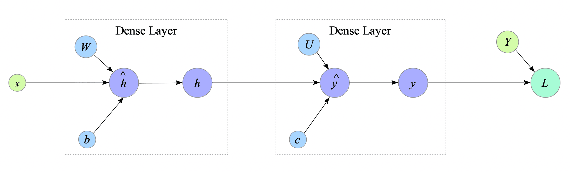
Fig.4-1: Two Elements in the XOR-Gate's Computational Graph
For an explanation of computational graphs, see Appendix 2.2.3.
Fig 4-2 illustrates a dense layer.
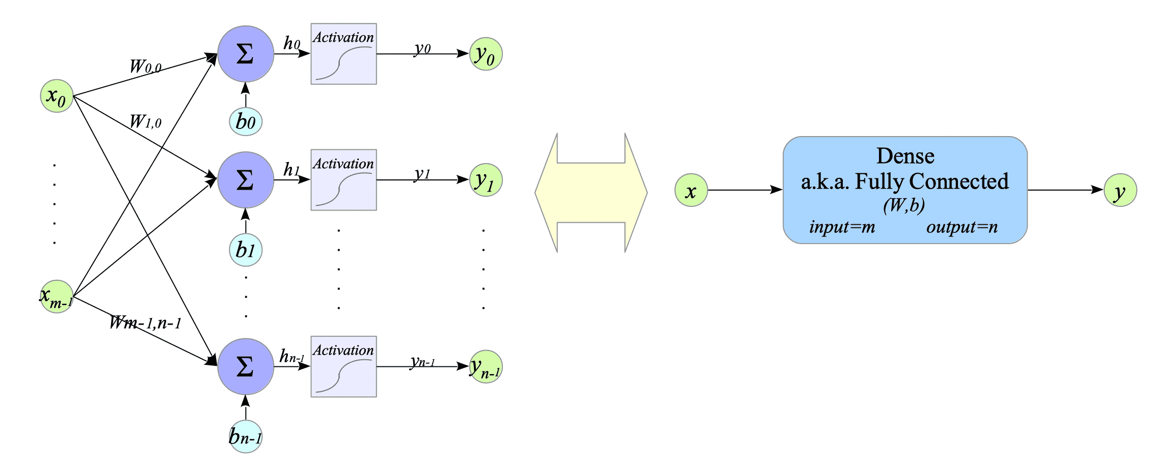
Fig.4-2: Dense Layer Architecture
Mathematically, a dense layer is defined as follows:
$$ \begin{cases} h = W x + b \\ y = f(h) \end{cases} $$where:
- $x \in \mathbb{R}^{m} $ is the input vector.
- $y \in \mathbb{R}^{n} $ is the output vector.
- $W \in \mathbb{R}^{n \times m} $ is the weight matrix.
- $b \in \mathbb{R}^{n} $ is the bias term.
- $f(\cdot)$ is an activation function.
Before computing the derivatives, we define the gradient $dL$ from a loss function $L$, which can be any loss function:
$$ dL \stackrel{\mathrm{def}}{=} \frac{\partial L}{\partial y} \\ $$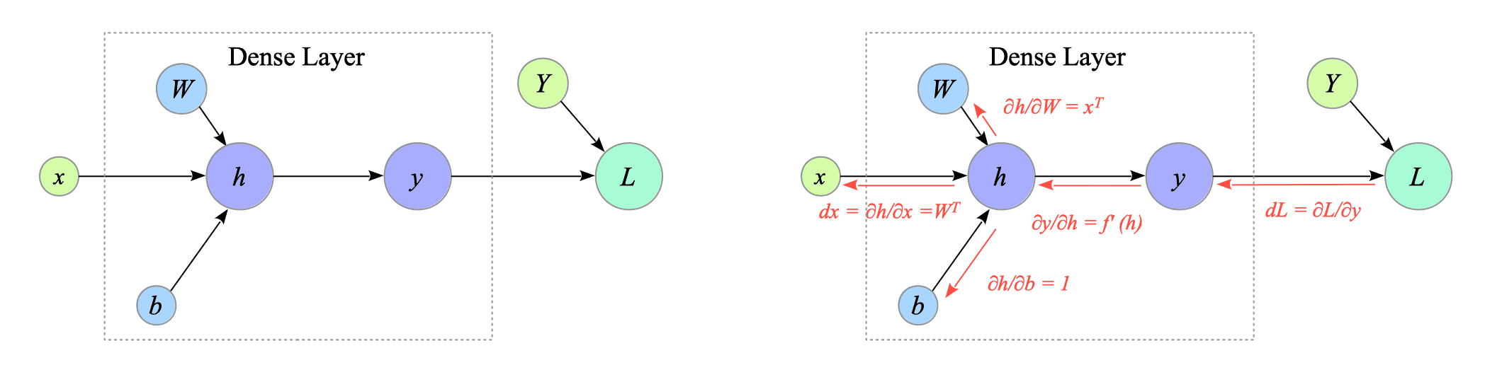
Fig.4-3: (Left) Forward Computational Graph of the Dense layer. (Right) Backward Computational Graph of the Dense layer.
Using this, we can derive the gradients $\frac{\partial L}{\partial b}, \frac{\partial L}{\partial W}$ and $\frac{\partial L}{\partial x}$ (denoted by $db, dW, dx$):
$$ \begin{align} db &\stackrel{\mathrm{def}}{=} \frac{\partial L}{\partial b} = \frac{\partial L}{\partial y} \frac{\partial y}{\partial h} \frac{\partial h}{\partial b} \\ &= f'(h) dL \\ dW &\stackrel{\mathrm{def}}{=} \frac{\partial L}{\partial W} = \frac{\partial L}{\partial y} \frac{\partial y}{\partial h} \frac{\partial h}{\partial W} \\ &= (f'(h) dL) x^{T} \\ &= db \ x^{T} \\ dx &\stackrel{\mathrm{def}}{=} \frac{\partial L}{\partial x} = \frac{\partial L}{\partial y} \frac{\partial y}{\partial h} \frac{\partial h}{\partial x} \\ &= W^{T} (f'(h) dL) \\ &= W^{T} \ db \end{align} $$$dx$ is the gradient that propagates to the next layer.
In this document, “$d$” denotes the gradient (e.g., $dL, dx$), not the total derivative.
4.1.1. Implementation
For complete implementation details, refer to the Layers.py.
Below is the Dense class:
#
# Dense Connection Layer, a.k.a. fully-connected Layer
#
class Dense:
    def __init__(self, input_size, output_size, activate_func=None, deriv_activate_func=None, activate_class=None):

        self.W = np.random.uniform(size=(output_size, input_size))
        self.b = np.random.uniform(size=(output_size, 1))

        self.activate_func = activate_func
        self.deriv_activate_func = deriv_activate_func
        self.activate_class = activate_class

    def get_grads(self):
        return [self.dW, self.db]

    def get_params(self):
        return [self.W, self.b]

    def num_params(self):
        return self.W.size + self.b.size

    def forward_prop(self, x):
        self.x = x
        self.h = np.dot(self.W, self.x) + self.b
        if self.activate_class == None:
            self.y = self.activate_func(self.h)
        else:
            self.y = self.activate_class.activate_func(self.h)
        return self.y

    def back_prop(self, grads):
        self.dW = np.zeros_like(self.W)
        self.db = np.zeros_like(self.b)

        if self.activate_class == None:
            self.db = self.deriv_activate_func(self.h) * grads
        else:
            self.db = self.activate_class.deriv_activate_func(self.h, grads)
        self.dW = np.dot(self.db, self.x.T)

        return np.dot(self.W.T, self.db)
The back_prop() method receives gradients from the next layer, calculates gradients for bias and weights, and returns the gradient to be propagated further back in the network.
The get_grads() and get_params() methods are used in the update_weights() function, explained in Section 6.3.
4.1.2. Remaking of XOR-gate
We remake XOR-gate.py to XOR-gate-modularized.py using the dense layer.
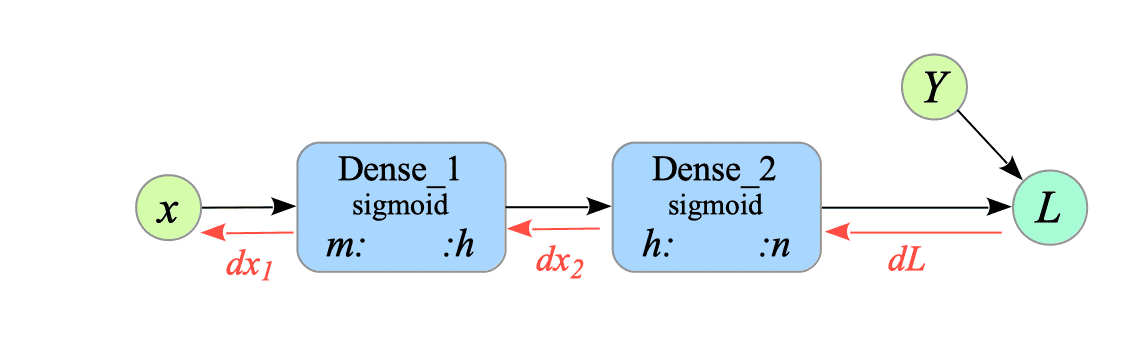
Fig.4-4: Pseudo-Computational Graph of XOR-gate with Dense Layers
[1] Prepare the inputs and the ground-truth labels.
# Inputs
X = np.array([[0, 0], [0, 1], [1, 0], [1, 1]])

# The ground-truth labels
Y = np.array([0, 1, 1, 0])

# Convert row vectors into column vectors.
X = X.reshape(4, 2, 1)
Y = Y.reshape(4, 1, 1)
[2] Create model
We create two dense layers: dense_1 and dense_2.
# ========================================
# Create Model
# ========================================

input_nodes = 2
hidden_nodes = 3
output_nodes = 1

dense_1 = Layers.Dense(input_nodes, hidden_nodes, sigmoid, deriv_sigmoid)
dense_2 = Layers.Dense(hidden_nodes, output_nodes, sigmoid, deriv_sigmoid)
[3] Training
The train() function explicitly builds the forward and backward propagation procedures.
In the forward propagation phase, the first dense layer (dencs_1) receives the input $x$ and outputs $y_{1}$, the second dense layer (dense_2) then receives $y_{1}$ as input and outputs $y$.
In the backward propagation phase, there are three steps:
- Compute $dL$. In this example, $dL = (y - Y)$ because the loss function is the mean squared error.
- Propagate the gradients backwards through the dense layers:
- The second dense layer receives $dL$ as input and outputs $dx_{2}$.
- The first dense layer receives $dx_{2}$ as input and outputs $dx_{1}$.
- Update the weights and biases of the dense layers. The update_weights() function is explained in Section 4.3.
# ========================================
# Training
# ========================================

def train(x, Y, lr=0.001):
    #
    # Forward Propagation
    #
    y1 = dense_1.forward_prop(x)
    y = dense_2.forward_prop(y1)

    #
    # Back Propagation
    #

    # 1st step
    loss = np.sum((y - Y) ** 2 / 2) # for measuring the training progress
    dL = (y - Y)

    # 2nd step
    dx2 = dense_2.back_prop(dL)
    dx1 = dense_1.back_prop(dx2)

    # 3rd step
    update_weights([dense_1, dense_2], lr=lr)

    return loss


n_epochs = 15000  # Epochs
lr = 0.1  # Learning rate

#
# Training loop
#
for epoch in range(1, n_epochs + 1):

    loss = 0.0

    for i in range(0, len(Y)):
        loss += train(X[i], Y[i], lr)
[4] Test
Run the following command to test the model:
$ python XOR-gate-modularized.py
_________________________________________________________________
 Layer (type)                Output Shape              Param #
=================================================================
 dense_1 (Dense)             (None,  3)                    9
 dense_2 (Dense)             (None,  1)                    4
=================================================================
Total params: 13

epoch: 1 / 15000  Loss = 0.826220
epoch: 1000 / 15000  Loss = 0.501673
epoch: 2000 / 15000  Loss = 0.457671
epoch: 3000 / 15000  Loss = 0.348954
epoch: 4000 / 15000  Loss = 0.176073
epoch: 5000 / 15000  Loss = 0.054048
epoch: 6000 / 15000  Loss = 0.023446
epoch: 7000 / 15000  Loss = 0.013698
epoch: 8000 / 15000  Loss = 0.009367
epoch: 9000 / 15000  Loss = 0.007011
epoch: 10000 / 15000  Loss = 0.005557
epoch: 11000 / 15000  Loss = 0.004580
epoch: 12000 / 15000  Loss = 0.003883
epoch: 13000 / 15000  Loss = 0.003363
epoch: 14000 / 15000  Loss = 0.002961
epoch: 15000 / 15000  Loss = 0.002642
------------------------
x0 XOR x1 => result
========================
 0 XOR  0 => 0.0319
 0 XOR  1 => 0.9756
 1 XOR  0 => 0.9551
 1 XOR  1 => 0.0406
========================
The model output indicates that it has learned the XOR gate functionality.