2.4. Probability

Probability is one of the mathematical concepts that many people are not good at. However, to understand Transformer model, only simple knowledge of discrete probability is required.

2.4.1. Probability

We learned in elementary school that the probability of rolling a $1$ on a standard die 🎲 is $1/6$. This is because a die has six sides, and we assume that all outcomes are equally likely.

Now, we represent that $\Omega$ as a finite set that contains all outcomes, and $x$ as an element of the set $\Omega$. In the above example, $\Omega = $ { $ x | x = 1, 2, 3, 4, 5, 6$ }.

Generally, if all outcomes in a finite set $\Omega$ are equally likely, the probability of $x$ is the number of outcomes in $x$ divided by the total number of outcomes:

When $x = 1$, $P(x = 1)$ can be obtained as follows:

2.4.1.1. Empirical Probability

In real-world scenarios, outcomes may not always be equally likely. The probability of an event can only be obtained by observation.

The probability based on observation is called the empirical probability. The empirical probability of an event is calculated by dividing the number of times the event occurred by the total number of trials:

I show an example using a virtual dice.

Here is the result of tossing this dice 30,000 times:

$ python Dice.py
========================================
P(Event) = |event|/|trial| = Probability
----------------------------------------
 P(1)    =>  5129 / 30000  = 0.17097
 P(2)    =>  4987 / 30000  = 0.16623
 P(3)    =>  5036 / 30000  = 0.16787
 P(4)    =>  5064 / 30000  = 0.16880
 P(5)    =>  4940 / 30000  = 0.16467
 P(6)    =>  4844 / 30000  = 0.16147
----------------------------------------

Using the result, we can calculate the probabilities of all possible events.

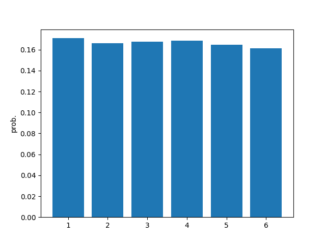
2.4.2. Conditional Probability

In probability theory, conditional probability, denoted by $P(x_{2} | x_{1})$, represents the probability of event $x_{2}$ occurring given that event $x_{1}$ has already happened.

For a finite set $\Omega $ of equally likely outcomes, and events $x_{1}$ and $x_{2}$ represented by subsets $\Omega$, the conditional probability of $x_{2}$ given $x_{1}$ is:

Example:

The simplest example is when we toss an ideal dice and get an odd number, then find the probability that it is $1$. In this case, event $x_{1} = $ {$x|x = 1,3,5 $} and event $x_{2} = $ {$x|x = 1$}, so $P(x_{1})$ and $P(x_{1} \cap x_{2})$ are as follows:

Therefore, $P(x_{2}|x_{1})$ is obtained as follows:

2.4.3. Chain Rule

There is also the chain rule in probability, so let’s derive it.

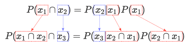
First, to obtain $P(x_{1} \cap x_{2})$, we multiply both sides of the conditional probability formula $(2.1)$ by $P(x_{1})$, so we get the following expression:

Next, to extend the expression $(2.2)$ to the three-variable version $P(x_{1} \cap x_{2} \cap x_{3})$, we can replace $x_{2}$ with $x_{3}$ and $x_{1}$ with $x_{1} \cap x_{2}$:

By performing similar operations recursively, we can obtain the chain rule shown below:

To simplify, the following notation is often used:

Using the introduced notation, the chain rule can be expressed as follows: