14.4. Encoder-Decoder with Attention
We build upon the encoder-decoder machine translation model, from Chapter 13, by incorporating an attention mechanism.
14.4.1. Implementation
Complete Python code is available at: seq2seq-tf-attention.py
14.4.1.1. Encoder
The encoder comprises a word embedding layer and a many-to-many GRU network.
-
Word Embedding Layer: The inputs $x$ passed through the word embedding layer before being fed into the GRU unit.
-
Many-to-Many GRU Layer: We set $\text{return_sequences}=\text{True}$ and $\text{return_state}=\text{True}$. This returns both the final hidden state ($\text{state}$) and the entire sequence of hidden states ($\text{output}$).
#
# Encoder
#
class Encoder(tf.keras.Model):
    def __init__(self, vocab_size, embedding_dim, enc_units, batch_sz):
        super(Encoder, self).__init__()
        self.batch_sz = batch_sz
        self.enc_units = enc_units
        self.embedding = tf.keras.layers.Embedding(vocab_size, embedding_dim)
        """
        Bahdanau attention model uses bidirectional RNN in the original paper,
        but we use a simple GRU.
        """
        self.gru = tf.keras.layers.GRU(
            self.enc_units,
            return_sequences=True,
            return_state=True,
            recurrent_initializer="glorot_uniform",
        )

    def call(self, x):
        x = self.embedding(x)
        output, state = self.gru(x)
        return output, state
14.4.1.2. Decoder
The decoder comprises a word embedding layer, a many-to-many GRU network, an attention layer and a Dense Layer with the Softmax activation function.
-
Word Embedding Layer and Many-to-Many GRU Layer: These layers are equivalent to the encoder.
-
Attention Layer: The decoder can employ either Luong or Bahdanau attention, depending on the setting of the AttentionType variable in the code:
The selected attention influences the decoder’s behavior. This will be explained in Section 14.4.3.AttentionType = "Bahdanau" # a.k.a. Additive attention, Multi-Layer perceptron. # AttentionType = "Luong" # a.k.a. Bilinear , General attention. -
Dense Layer: Its output size equals the size of the vocabulary, providing probabilities for each word in the vocabulary.
#
# Decoder
#
class Decoder(tf.keras.Model):
    def __init__(self, vocab_size, embedding_dim, dec_units, batch_sz):
        super(Decoder, self).__init__()
        self.batch_sz = batch_sz
        self.dec_units = dec_units
        self.embedding = tf.keras.layers.Embedding(vocab_size, embedding_dim)
        self.gru = tf.keras.layers.GRU(
            self.dec_units,
            return_sequences=True,
            return_state=True,
            recurrent_initializer="glorot_uniform",
        )
        self.softmax = tf.keras.layers.Dense(vocab_size, activation="softmax")

        if AttentionType == "Bahdanau":
            self.attention = Attention.BahdanauAttention(self.dec_units)
        elif AttentionType == "Luong":
            self.attention = Attention.LuongAttention(self.dec_units)
            self.W = tf.keras.layers.Dense(2 * units)
        else:
            print("Error: {} is not supported.".format(Attention))
            sys.exit()

    def call(self, x, hidden, enc_output):
        x = self.embedding(x)

        if AttentionType == "Bahdanau":
            context_vector, attention_weights = self.attention(hidden, enc_output)
            x = tf.concat([tf.expand_dims(context_vector, 1), x], axis=-1)
            output, state = self.gru(inputs=x)
            output = tf.reshape(output, (-1, output.shape[2]))
        else:
            """ Luong """
            output, state = self.gru(inputs=x, initial_state=hidden)
            context_vector, attention_weights = self.attention(state, enc_output)
            output = tf.nn.tanh(self.W(tf.concat([state, context_vector], axis=-1)))

        x = self.softmax(output)

        return x, state, attention_weights
14.4.2. Training
The training function $\text{train}()$ is similar to the one without attention, explained in Section 13.2.3. However, there are two key differences:
-
Encoder Output: The encoder returns not only the context vector but also all its hidden layer outputs. These outputs are passed to the attention layer.
-
Decoder Processing: Due to limitations of the attention layer, the decoder processes one token at a time.
Here’s the updated training function:
@tf.function
def train(encoder, decoder, source_sentences, target_sentences, target_lang_tokenizer):

    with tf.GradientTape() as tape:
        enc_output, context_vector = encoder(source_sentences)

        predictions = decoder_training(decoder, enc_output, context_vector, target_sentences, target_lang_tokenizer)

        expected_dec_output = target_sentences[:, 1:]
        loss = loss_function(expected_dec_output, predictions)
        train_accuracy(expected_dec_output, predictions)

    batch_loss = loss / int(target_sentences.shape[1])
    variables = encoder.variables + decoder.variables
    gradients = tape.gradient(loss, variables)

    optimizer.apply_gradients(zip(gradients, variables))

    return batch_loss

#
# To avoid overfitting, limit training duration when using this model.
# In my experience, it performs well after around 7 epochs.
#
# If n_epochs = 0, this model uses the trained parameters saved in the last checkpoint,
# allowing you to perform machine translation without retraining.
if len(sys.argv) == 2:
    n_epochs = int(sys.argv[1])
else:
    n_epochs = 7

for epoch in range(1, n_epochs + 1):
    start = time.time()

    total_loss = 0
    train_accuracy.reset_states()

    for (batch, (source_sentences, target_sentences)) in enumerate(dataset):

        batch_loss = train(encoder, decoder, source_sentences, target_sentences, target_lang_tokenizer)
        total_loss += batch_loss
Since the attention layer only processes one token ($\text{dec_input}$) at a time, we need to feed tokens to the decoder sequentially.
Therefore, we force our GRU-based decoder to behave like a “One-to-One” RNN and explicitly iterate the single decoder step. This involves passing the previous hidden state ($\text{dec_hidden}$) as input to the next step, resulting in the decoder working as a “Many-to-Many” RNN.
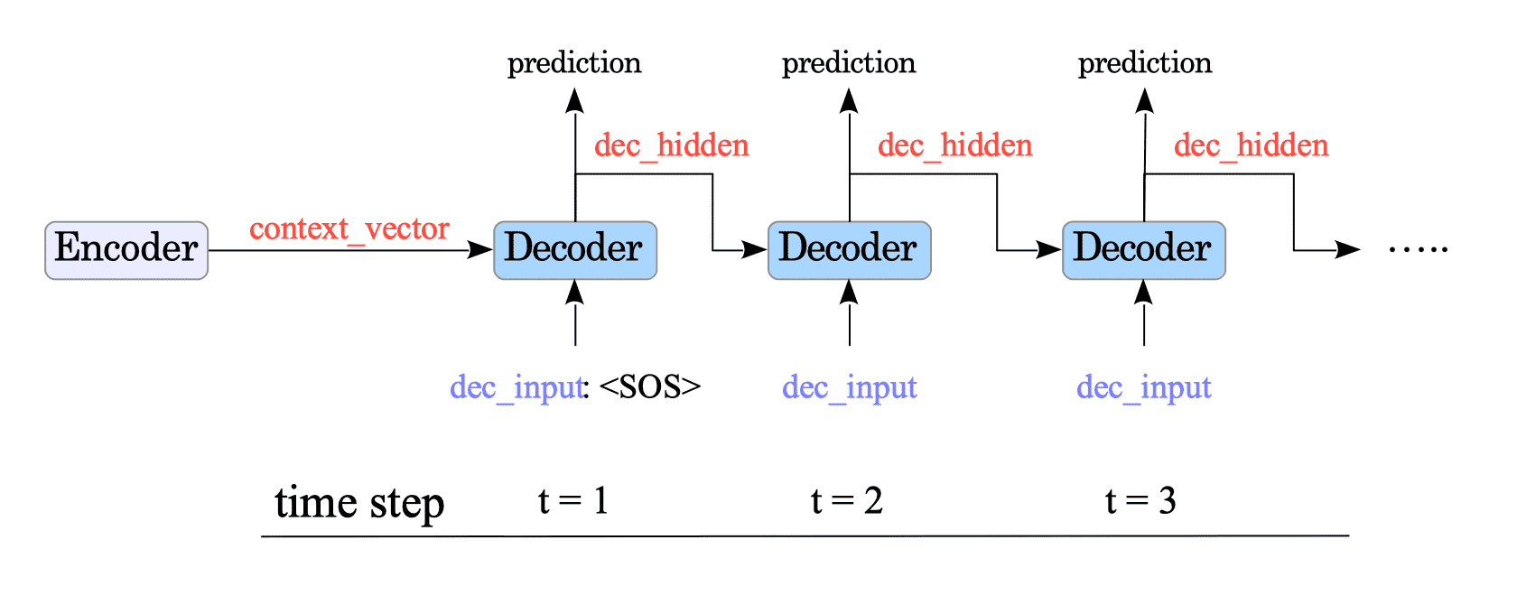
Fig.14-6: Decoding Process with Attention Mechanism
The $\text{decoder_training}()$ function is a wrapper that hides this token-by-token processing functionality:
@tf.function
def decoder_training(decoder, enc_output, context_vector, target_sentences, target_lang_tokenizer):

    dec_hidden = context_vector

    # Set the initial token.
    dec_input = tf.expand_dims([target_lang_tokenizer.word2idx["<SOS>"]] * BATCH_SIZE, 1)

    #
    for t in range(1, target_sentences.shape[1]):
        expected_next_token = target_sentences[:, t]
        prediction, dec_hidden, _ = decoder(dec_input, dec_hidden, enc_output)

        if t == 1:
            predictions = tf.concat([tf.expand_dims(prediction, axis=1)], axis=1)
        else:
            predictions = tf.concat([predictions, tf.expand_dims(prediction, axis=1)], axis=1)

        # Retrieve the next token.
        dec_input = tf.expand_dims(expected_next_token, 1)

    return predictions
14.4.3. Translation
During translation, the decoder leverages the attention layer to understand the context of the source sentence and predict words more accurately.
Depending on the selected attention style, the way the attention layer calculates the context vector differs.
14.4.3.1. Bahdanau attention
In Bahdanau attention, when predicting the word at time step $t$, the query $q_{t}$ is the previous hidden state $h^{(t-1)}$ of the GRU unit.
(For the first word ($t=1$), the query $q_{1}$ is the final hidden state of the encoder.)
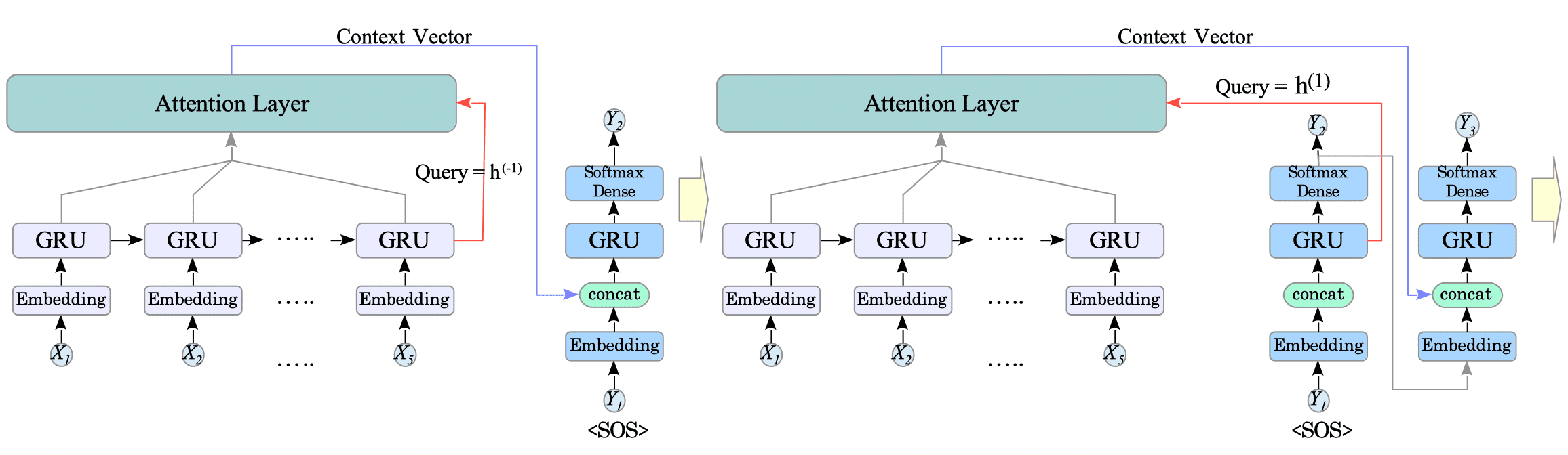
Fig.14-7: Translation with Bahdanau Attention
The context vector is then concatenated with the embedded input before feeding them jointly to the GRU unit.
This allows the GRU to directly incorporate the contextual information into its hidden state update.
14.4.3.1.1. Attention Weight Map
When our model translates a Spanish sentence to an English sentence, it also shows an attention weight map.
For example, when the sentence “Soy Hironobu.” is fed to the model, it returns the translated sentence “I’m Hironobu.” and shows the following attention weight map.
- Source: “Soy Hironobu.” $\Longrightarrow$ Target: “I’m Hironobu.”
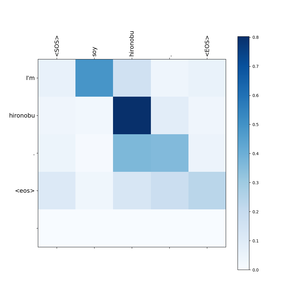
Each row in the attention weight map represents the attention weights that was used to predict the corresponding word in the translated sentence.
For instance, the first row of the map above visualizes the attention weight that was used to predict the first word “I’m.”
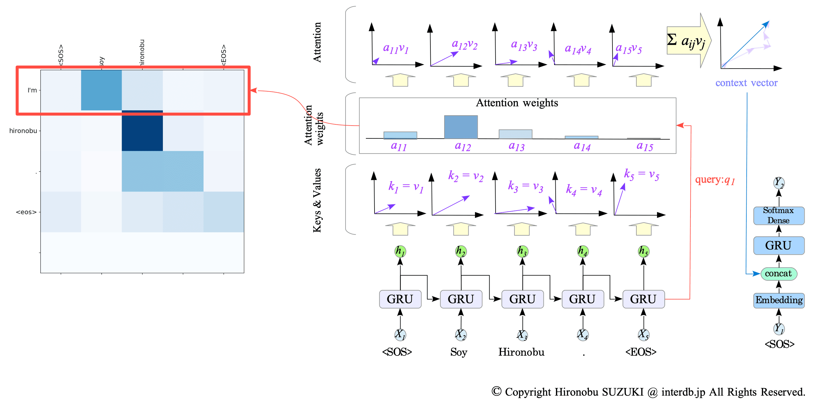
Fig.14-8: Attention Weight Map and Translation Process
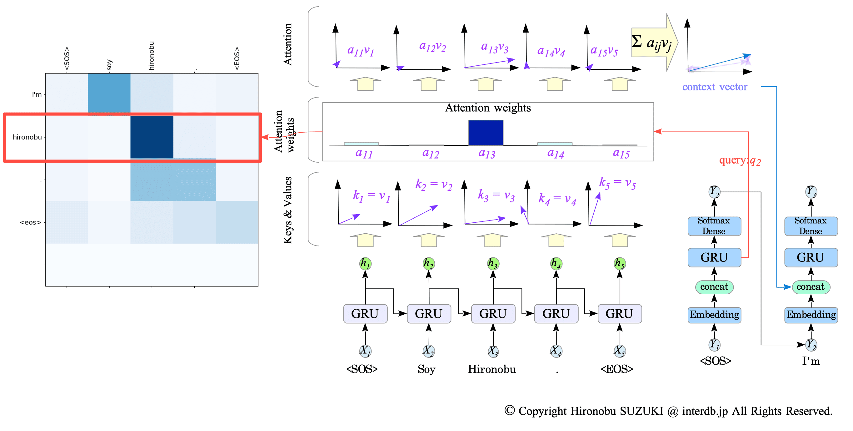
Fig.14-9: Attention Weight Map and Translation Process (cont.)
14.4.3.2. Luong attention
In Luong attention, when predicting the word at time step $t$, the query $q_{t}$ is the hidden state $h^{(t)}$ of the GRU that processed the input at time step $t$.
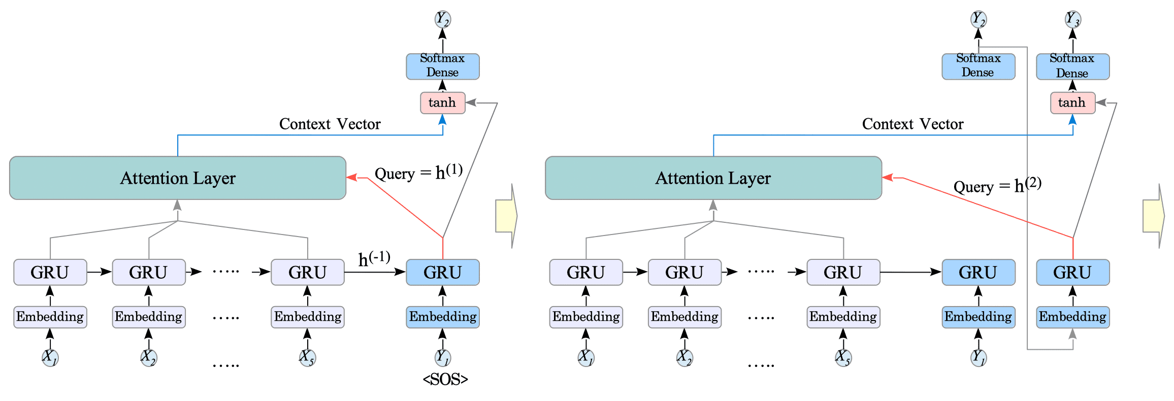
Fig.14-10: Translation with Luong Attention
The GRU’s state $h^{(t)}$ and the context vector from the attention layer are then combined using $concat()$ function and fed through a $\tanh$ activation function:
$$ \text{output} = \tanh(W( concat([\text{state}, \text{context_vector}])) $$where
- $concat([\text{state}, \text{context_vector}])$ combines the decoder’s $\text{state}$ (same as the query) and the $\text{context_vector}$.
- $W$ is a weight matrix responsible for learning the importance of different elements in the combined vector.
The resulting output is then fed to the softmax layer for predicting the next word.
14.4.4. Demonstration
Following 7 epochs of training, here are some examples of our model’s translation outputs:
To avoid overfitting, limit training duration when using this model. In my experience, it performs well after around 7 epochs.
$ python seq2seq-tf-attention.py
===== [1] ======
Input : nosotros le mostramos algunas fotos de los alpes.
Predicted: We showed him some pictures of the alps . <eos>
Correct : we showed him some pictures of the alps.
===== [2] ======
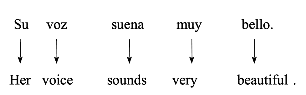
Input : su voz suena muy bello.
Predicted: Her voice sounds very beautiful . <eos>
Correct : her voice sounds very beautiful.
===== [3] ======
Input : pense que no conocias a tom.
Predicted: I thought you didn't know tom . <eos>
Correct : i thought you didn't know tom.
===== [4] ======
Input : no nos gusta la lluvia.
Predicted: We don't like rain . <eos>
Correct : we don't like rain.
===== [5] ======
Input : ven por aqui.
Predicted: Come over here . <eos>
Correct : walk this way.
===== [6] ======
Input : eres su hermano, ¿ verdad ?
Predicted: You're his brother , right ? <eos>
Correct : you are his brother, right ?
===== [7] ======
Input : tom charlo.
Predicted: Tom will go down . <eos>
Correct : tom talked.
===== [8] ======
Input : ojala tuviera un coche.
Predicted: I wish i had a car . <eos>
Correct : i wish i had a car.
===== [9] ======
Input : tom pretende ser mas cuidadoso en el futuro.
Predicted: Tom plans to be more careful in the future . <eos>
Correct : tom plans to be more careful in the future.
===== [10] ======
Input : hace anos que vivo aqui.
Predicted: I have lived here for years . <eos>
Correct : i have been living here for years.This code contains the checkpoint function that preserves the training progress. Hence, once trained, the task can be executed without retraining by setting the parameter $\text{n_epochs}$ to $0$, or simply passing $0$ when executing the Python code, as shown below:
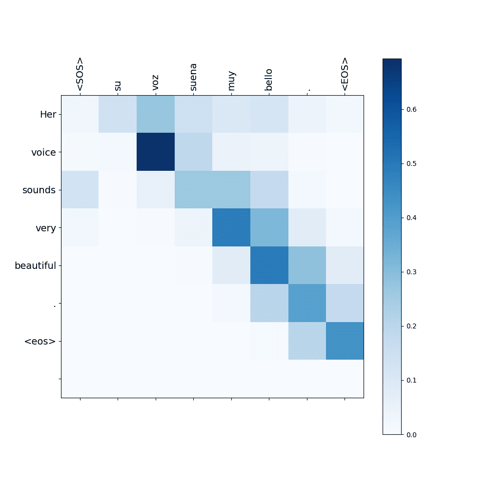
$ python seq2seq-tf-attention.py 0Examining three specific attention weights from the results, we observe that the model accurately translates the sentences while the attention weights effectively reflect word relationships across contexts in Spanish and English.
- Source: “Su voz suena muy bello.” $\Longrightarrow$ Target: “Her voice sounds very beautiful.”
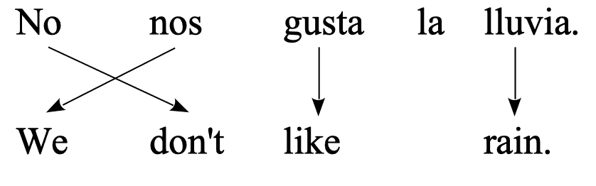
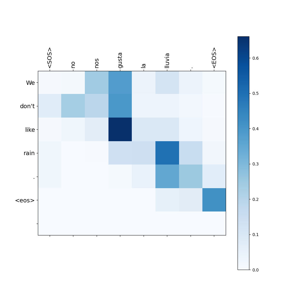
- Source: “No nos gusta la lluvia.” $\Longrightarrow$ Target: “We don’t like rain."
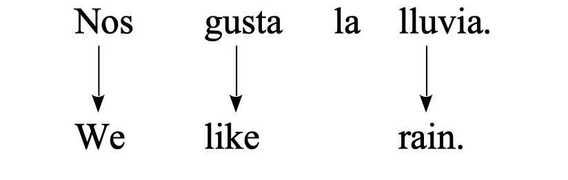
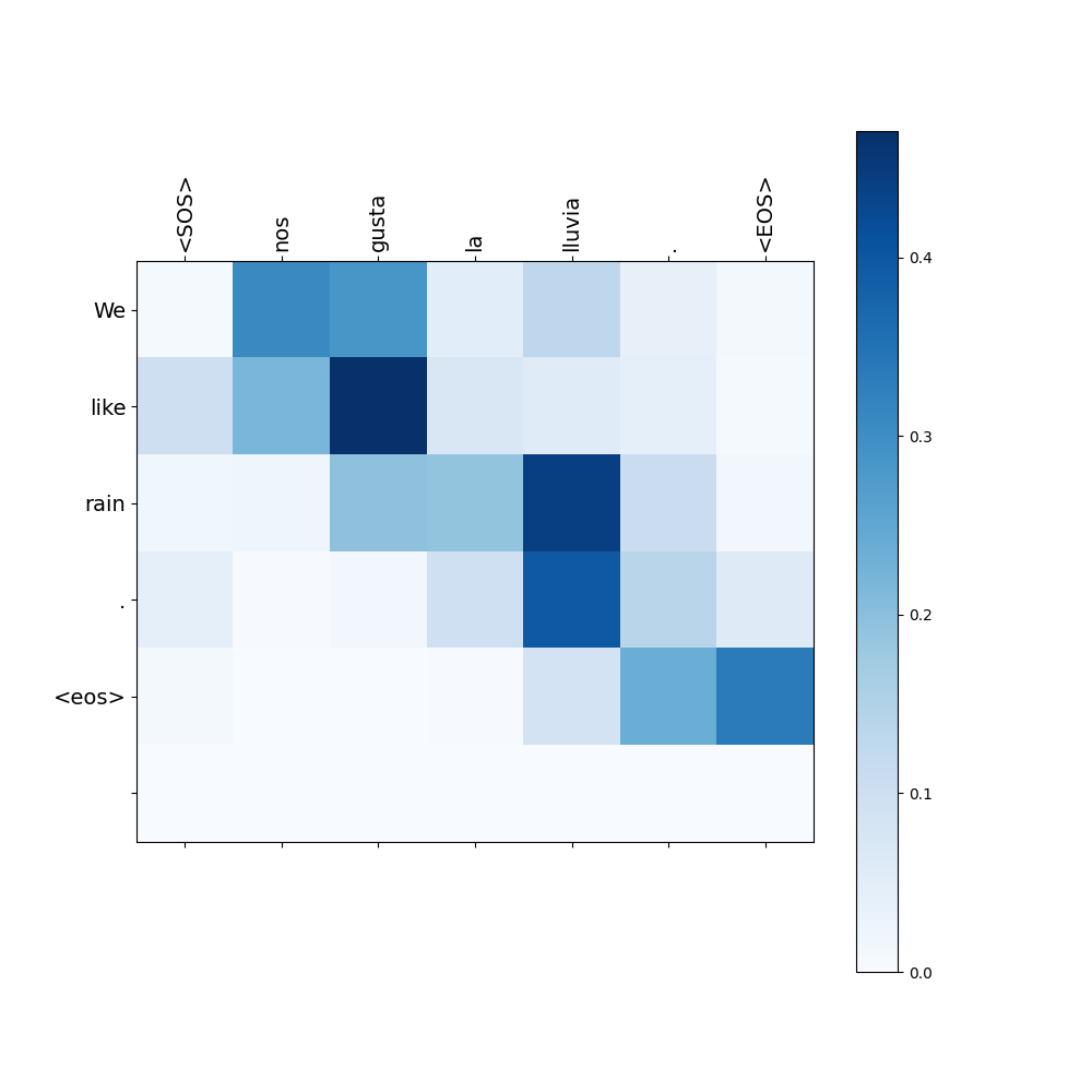
Source: “Nos gusta la lluvia.” $\Longrightarrow$ Target: “We like rain."
These examples demonstrate that the attention mechanism goes beyond simply replacing words with high similarity scores one after another sequentially. Instead, it learns the relationships between words in different languages and the context within those languages.