4.2. Softmax Activation Function
Previously, we approached the XOR gate learning task as a single-variable classification problem. Now, we will tackle it as a binary classification problem, leveraging the softmax function as the activation function.
The softmax function is defined as:
$$ y_{i} = \frac{ \exp(h_{i}) }{ \sum^{n-1}_{k=0} \exp(h_{k}) } \tag{4.1} $$where:
- $n \in \mathbb{N}$ is the number of category.
- $y_{i}$ is the $i$-th element of the output vector $y \in \mathbb{R}^{n}$. It satisfies $\sum_{i=0}^{n-1} y_{i} = 1$ and $ y_{i} \in [0, 1]$.
- $h_{i}$ is the $i$-th element of the input vector $h \in \mathbb{R}^{n}$.
The detail is explained in Section 3.2.2.
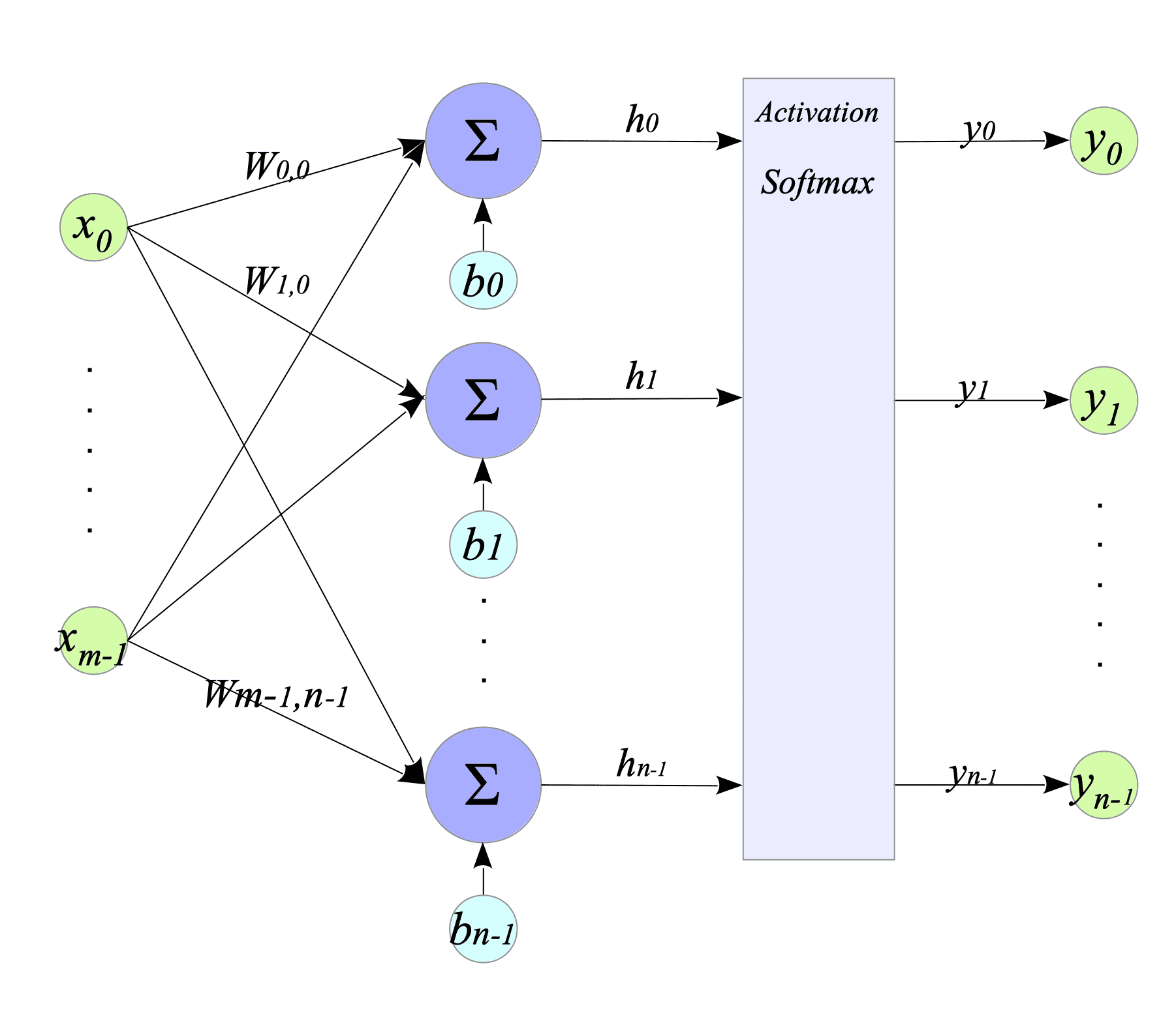
Fig.4-5: Dense Layer with Softmax Activation Function
4.2.1. Computing the gradients for Back Propagation
To obtain the gradient of the softmax function, we will use the cross-entropy (CE) as the loss function. The CE is defined as follows:
$$ L = - \sum^{n-1}_{i=0} Y_{i} \log(y_{i}) \tag{4.2} $$where:
- $n$ is the number of category.
- $Y_{i} \in $ { $0,1$ } is the ground-truth label for the $i$-th data point. If $Y_{i} = 1$ (truth), then all other $Y_{j} = 0$ for $j \neq i$.
- $y_{i} \in [0,1]$ is the predicted probability for the $i$-th data point.
The term $\sum_{i=0}^{n-1} Y_{i} = 1$ is by definition, because the ground-truth labels must sum to 1.
First, we calculate $dL_{i} \stackrel{\mathrm{def}}{=} \dfrac{\partial L}{\partial y_i}$, which is the gradient propagated to the softmax function.
$$ \begin{align} dL_{i} = \frac{\partial L}{\partial y_{i}} = \dfrac{\partial}{\partial y_i} \left[ -\sum_{j=0}^{n-1} Y_j \log(y_j) \right] = -\sum_{j=0}^{n-1} Y_j \dfrac{\partial \log(y_j)}{\partial y_i} = -\dfrac{Y_i}{y_i} \end{align} \tag{4.3} $$Next, we calculate $ \partial L / \partial h_{k} $, which is the gradient propagated from the softmax function to the dense layer.
$$ \begin{align} \frac{\partial L}{\partial h_{k}} &= - \sum^{n-1}_{j=0} Y_{j} \frac {\partial \log(y_{j}) }{\partial h_{k}} = - \sum^{n-1}_{j=0} Y_{j} \frac {\partial \log(y_{j}) }{\partial y_{j}} \frac {\partial y_{j} }{\partial h_{k}} = - \sum^{n-1}_{j=0} \frac{Y_{j}} {y_{j}} \frac {\partial y_{j} }{\partial h_{k}} \end{align} \tag{4.4} $$Here we can calculate $\partial y / \partial h$ using the formula: $ d(\frac{f(x)}{g(x)})/dx = \frac{f’(x)g(x)-f(x)g’(x)}{g(x)^{2}}$.
$$ \begin{align} \frac{\partial y_{j}}{\partial h_{k}} &= \frac{\partial}{\partial h_{k}} \left[ \frac{\exp(h_{j})}{\sum_{i=0}^{n-1} \exp(h_{i})} \right] \\ &= \frac{1}{\left( \sum_{i=0}^{n-1} \exp(h_{i})\right)^{2}} \left[ \frac{\partial \exp(h_{j})}{\partial h_{k}} \sum_{i=0}^{n-1} \exp(h_{i}) - \exp(h_{j}) \frac{\partial}{\partial h_{k}} \left( \sum_{i=0}^{n-1} \exp(h_{i}) \right) \right] \\ &= \frac{1}{\left( \sum_{i=0}^{n-1} \exp(h_{i}) \right)^{2}} \left[ \delta_{j,k} \exp(h_{j}) \sum_{i=0}^{n-1} \exp(h_{i}) - \exp(h_{j}) \exp(h_{k}) \right] \\ &= \delta_{j,k} \frac{\exp(h_{j})}{\sum_{i=0}^{n-1} \exp(h_{i})} - \frac{\exp(h_{j})}{\sum_{i=0}^{n-1} \exp(h_{i})} \frac{\exp(h_{k})}{\sum_{i=0}^{n-1} \exp(h_{i})} \\ &= \delta_{j,k} y_{j} - y_{j} y_{k} \end{align} \tag{4.5} $$where $\delta_{j,k}$ is the Kronecker delta, which is equal to $1$ if $j=k$ and $0$ otherwise.
Using $(4.3),(4.4)$ and $(4.5)$, we finally obtain the following result:
$$ \begin{align} \frac{\partial L}{\partial h_{k}} &= - \sum^{n-1}_{j=0} \frac{Y_{j}} {y_{j}} (\delta_{j,k} y_{k} - y_{j}y_{k}) = \sum^{n-1}_{j=0} \left[ Y_{j} y_{k} - \delta_{j,k} \frac{Y_{j}}{y_{j}} y_{k} \right] \\ &= y_{k} \left[ \sum^{n-1}_{j=0} Y_{j} + \sum^{n-1}_{j=0} \delta_{j,k} \left( - \frac{Y_{j}}{y_{j}} \right) \right] = y_{k} \left[ 1 + \left( - \frac{Y_{k}}{y_{k}} \right) \right] \\ &= y_{k} (1 + dL_{k}) \end{align} \tag{4.6} $$4.2.2. Softmax Class
Complete Python code is available at: ActivationFunctions.py
The Python class below encapsulates the softmax activation function:
#
# Softmax
#
# Assume that the loss function is the Cross-Entropy (CE).
#
class Softmax:

    def activate_func(self, x):
        exp = np.exp(x)
        self.y = exp / (np.sum(exp, axis=0) + 1e-8)
        return self.y

    # dL should be (- Label / output) because of CE.
    def deriv_activate_func(self, _, dL):
        return self.y * (1 + dL)
This activation function assumes the model employs the CE loss function.
4.2.3. Implementation
This subsection showcases two applications using the softmax activation function:
- XOR-gate
- Binary-to-Decimal conversion
4.2.3.1. Implementing XOR-gate
We implement a XOR-gate model as a binary classified problem using softmax function.
Complete Python code is available at: XOR-gate-softmax.py
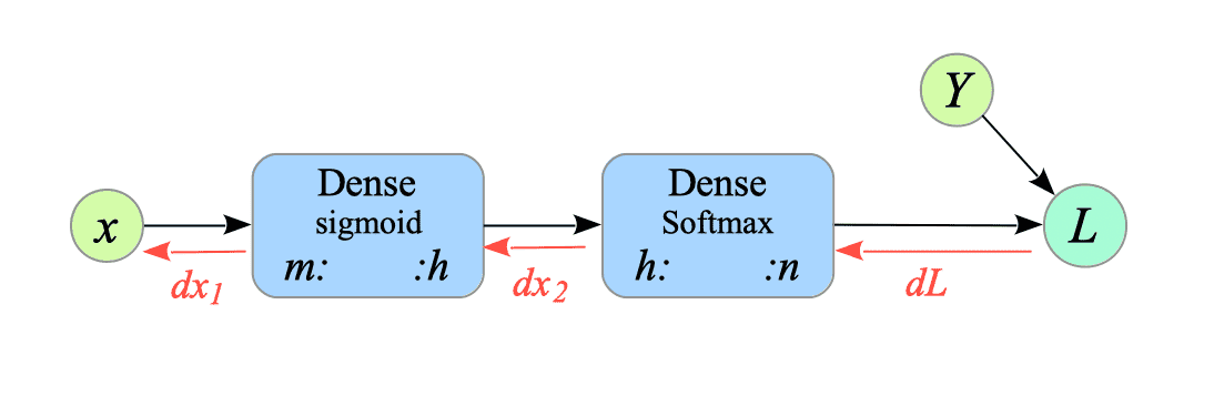
Fig.4-6: Pseudo-Computational Graph of XOR-gate with Dense Layers (Sigmoid and Softmax).
[1] Prepare the inputs and the ground-truth labels.
To handle the task as a classification task, which requires categorical input data, we need to convert the ground truth data $Y$ into one-hot vectors.
# ========================================
# Create datasets
# ========================================

# Inputs
X = np.array([[0, 0], [0, 1], [1, 0], [1, 1]])

# The ground-truth labels
Y = np.array([[0], [1], [1], [0]])


# Convert into One-Hot vector
Y = keras.utils.to_categorical(Y, 2)

"""
Y= [[1. 0.]
    [0. 1.]
    [0. 1.]
    [1. 0.]]
"""

# Convert row vectors into column vectors.
X = X.reshape(4, 2, 1)
Y = Y.reshape(4, 2, 1)
[2] Create model.
We create a dense layer and a softmax layer.
# ========================================
# Create Model
# ========================================

input_nodes = 2
hidden_nodes = 3
output_nodes = 2

dense = Layers.Dense(input_nodes, hidden_nodes, sigmoid, deriv_sigmoid)
softmax = Layers.Dense(hidden_nodes, output_nodes, activate_class=Softmax())
[3] Training.
The training phase remains largely the same as the neural network with double dense layers, with the key difference being the loss function used.
Our softmax activation function assumes the cross-entropy function $L$, defined in expression $(4.2)$, as loss function. Therefore, we utilize the gradient of this loss function $dL_{i}$ given by expression $(4.3)$.
def train(x, Y, lr=0.001):

    # Forward Propagation
    y = dense.forward_prop(x)
    y = softmax.forward_prop(y)

    # Back Propagation
    loss = -np.sum(Y * np.log(y + 1e-8)) # for measuring the training progress

    dL = - Y / (y + 1e-8)
    dx = softmax.back_prop(dL)
    _ = dense.back_prop(dx)

    # Weights and Bias Update
    update_weights([dense, softmax], lr=lr)

    return loss

n_epochs = 15000  # Epochs
lr = 0.1  # Learning rate

#
# Training loop
#
for epoch in range(1, n_epochs + 1):

    loss = 0.0

    for i in range(0, len(Y)):
        loss += train(X[i], Y[i], lr)
[4] Test.
Run the following command to test the model:
$ python XOR-gate-softmax.py
_________________________________________________________________
Layer (type) Output Shape Param #
=================================================================
dense (Dense) (None, 3) 9
softmax (Softmax) (None, 2) 8
=================================================================
Total params: 17
epoch: 1 / 15000 Loss = 3.108775
epoch: 1000 / 15000 Loss = 0.642858
epoch: 2000 / 15000 Loss = 0.046528
epoch: 3000 / 15000 Loss = 0.022903
epoch: 4000 / 15000 Loss = 0.015087
epoch: 5000 / 15000 Loss = 0.011222
epoch: 6000 / 15000 Loss = 0.008922
epoch: 7000 / 15000 Loss = 0.007400
epoch: 8000 / 15000 Loss = 0.006319
epoch: 9000 / 15000 Loss = 0.005512
epoch: 10000 / 15000 Loss = 0.004887
epoch: 11000 / 15000 Loss = 0.004388
epoch: 12000 / 15000 Loss = 0.003982
epoch: 13000 / 15000 Loss = 0.003644
epoch: 14000 / 15000 Loss = 0.003358
epoch: 15000 / 15000 Loss = 0.003114
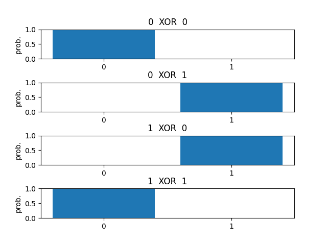
-------------------------------------
x0 XOR x1 => prob(0) prob(1)
=====================================
0 XOR 0 => 0.9998 0.0002
0 XOR 1 => 0.0009 0.9991
1 XOR 0 => 0.0008 0.9992
1 XOR 1 => 0.9987 0.0013
=====================================
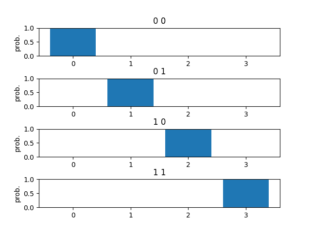
4.2.3.2. Implementing binary-to-decimal conversion model
This example demonstrates the versatility of neural networks.
By simply modifying the label data and the number of output node, we can transform the XOR gate model into a binary-to-decimal converter.
Complete Python code is available at: binary-to-decimal-conversion.py
# ========================================
# XOR-gate
# ========================================

Y = np.array([[0], [1], [1], [0]])

Y = keras.utils.to_categorical(Y, 2)

"""
Y= [[1. 0.]
    [0. 1.]
    [0. 1.]
    [1. 0.]]
"""

output_nodes = 2
# ========================================
# Binary-to-Decimal conversion
# ========================================
Y = np.array([[0], [1], [2], [3]])
Y = keras.utils.to_categorical(Y, 4)
"""
Y = [[1. 0. 0. 0.]
[0. 1. 0. 0.]
[0. 0. 1. 0.]
[0. 0. 0. 1.]]
"""
output_nodes = 4We can test its ability to convert binary to decimal numbers using the following command:
$ python binary-to-decimal-conversion.py
_________________________________________________________________
 Layer (type)                Output Shape              Param #
=================================================================
 dense (Dense)               (None,  3)                    9
 softmax (Softmax)           (None,  4)                   16
=================================================================
Total params: 25

epoch: 1 / 15000  Loss = 6.055010
epoch: 1000 / 15000  Loss = 0.087320
epoch: 2000 / 15000  Loss = 0.038823
epoch: 3000 / 15000  Loss = 0.024832
epoch: 4000 / 15000  Loss = 0.018224
epoch: 5000 / 15000  Loss = 0.014383
epoch: 6000 / 15000  Loss = 0.011874
epoch: 7000 / 15000  Loss = 0.010107
epoch: 8000 / 15000  Loss = 0.008797
epoch: 9000 / 15000  Loss = 0.007787
epoch: 10000 / 15000  Loss = 0.006984
epoch: 11000 / 15000  Loss = 0.006330
epoch: 12000 / 15000  Loss = 0.005789
epoch: 13000 / 15000  Loss = 0.005332
epoch: 14000 / 15000  Loss = 0.004942
epoch: 15000 / 15000  Loss = 0.004605
-------------------------------------------
(x0 x1) => prob(0) prob(1) prob(2) prob(3)
===========================================
(0   0) => 0.9989  0.0008  0.0003  0.0000
(0   1) => 0.0007  0.9989  0.0000  0.0005
(1   0) => 0.0003  0.0000  0.9988  0.0009
(1   1) => 0.0000  0.0005  0.0007  0.9989
===========================================