15.1. Positional Encoding
To simplify the discussion, we will focus on the encoder, however, the essence of the discussion can apply to the decoder as well.
An RNN-based encoder requires $N$ steps to process an $N$-word sentence, because the RNN sequentially processes the input sentence one word at a time. This can take a long time for long sentences.
In contrast, the Transformer’s encoder processes the entire input sentence at once, which can significantly reduce encoder processing time compared to RNN-based models. See Fig.15-4.
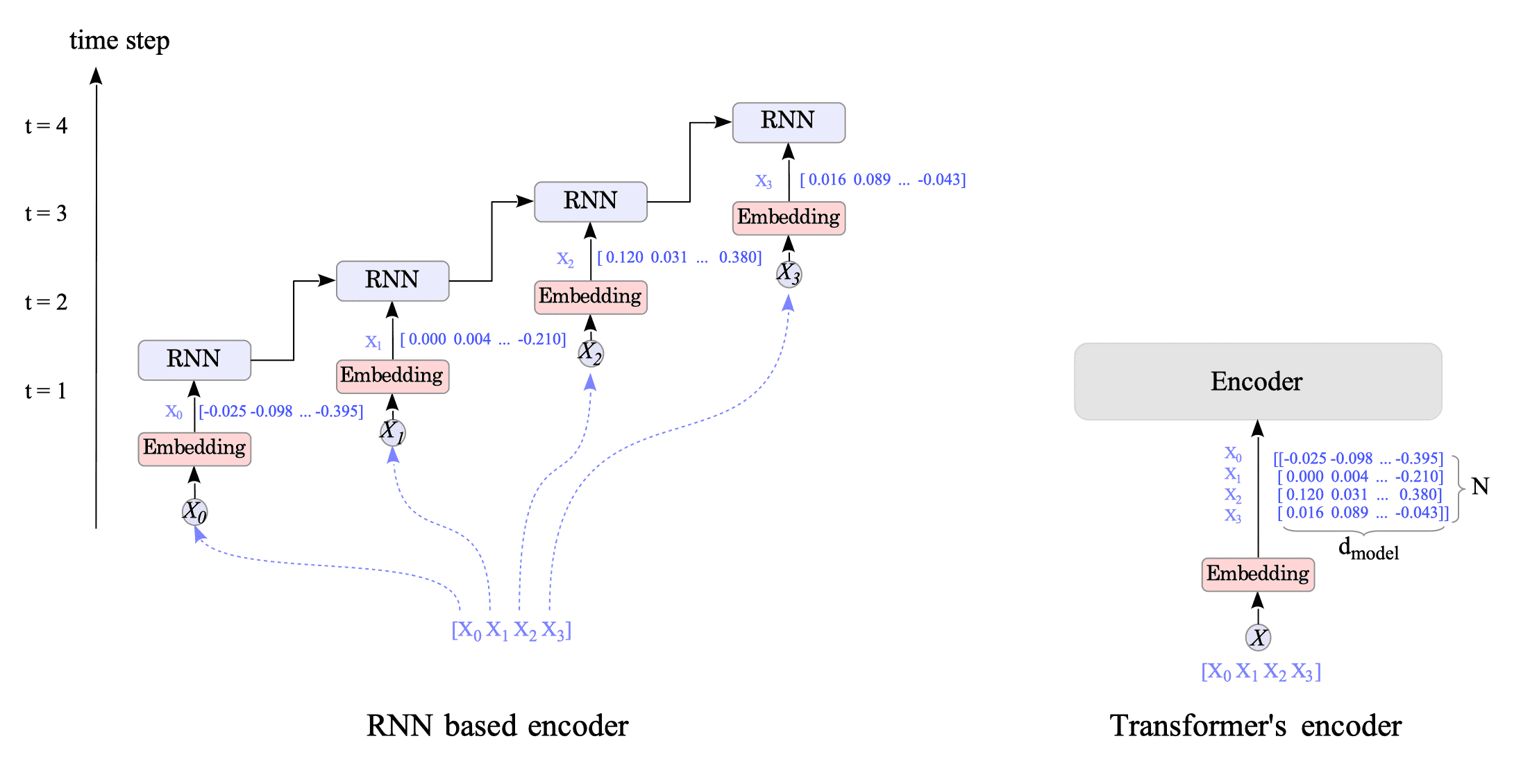
Fig.15-4: Comparison of RNN-Based Encoder vs. Transformer Encoder
Figure 15-4 shows a sentence with only four words. Imagine how much processing time could be reduced if a sentence with 512 or 1024 words were processed.
RNN-based encoders can theoretically accept sentences of infinite length. In contrast, the original Transformer cannot handle sentences longer than the maximum number of words $N$ set in the hyper-parameter.
This is one of the biggest shortcomings of the original Transformer model, for which improvements have been proposed. The issue is discussed in more detail in Section 17.1.
However, the Transformer’s encoder (and decoder) does not preserve the word order of the input sentence. For example, the encoder cannot distinguish between the sentences “John likes Jane” and “Jane likes John”. This is (also) a big problem, because word order is essential for meaning in all natural languages.
To address this problem, the authors of the Transformer paper introduced a technique called (absolute sinusoidal) positional encoding. This technique directly adds vector data to each embedded word that depends on the word’s position.
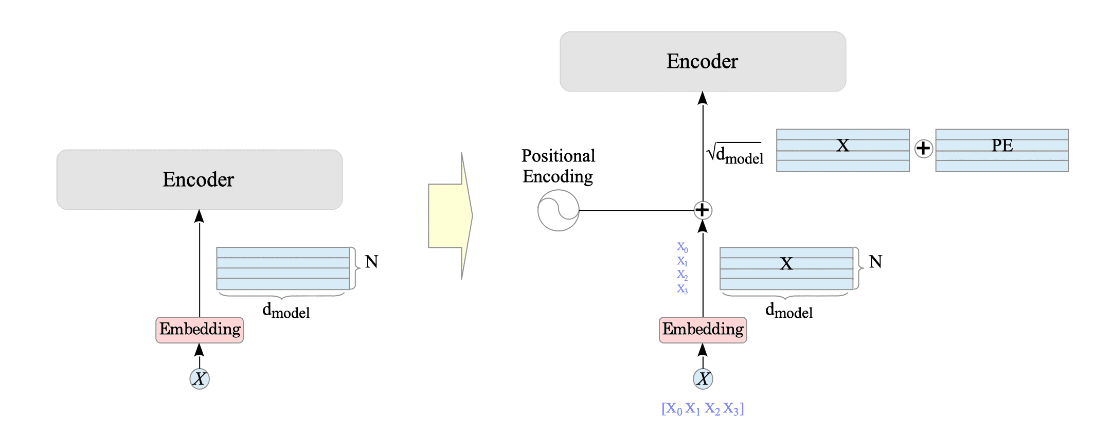
Fig.15-5: Transformer's Positional Encoding Mechanism
The following expression is the positional encoding of the original Transformer model:
$$ \begin{align} \text{PE}(pos, 2j) &= \sin \left( \frac{pos}{10000^{2j / d_{model}}} \right) \\ \text{PE}(pos, 2j+1) &= \cos \left( \frac{pos}{10000^{2j / d_{model}}} \right) \end{align} \tag{15.1} $$where:
- $ pos \in $ { $0,…, N-1$ } is the position.
- $ j \in $ { $0, …, \frac{d_{model}}{2} - 1$ } is the dimension.
I recommend to visit the following site, which provide visualizations of the original Transformer encoding:
In the original transformer, the input $X_{pe}$ is given by:
$$ X_{pe}(pos, i) = \sqrt{d_{model}} \cdot X_{em}(pos, i) + \text{PE}(pos, i) \tag{15.2} $$where $ i \in $ { $0, …,d_{model} - 1$ }, and a scaling factor $\sqrt{d_{model}}$ applied to the embedded input $X_{em}$.
The word embedding layer of the Transformer contains a learnable weight matrix $W_{e}$. Consequently, the embedded input $X_{em}$ is computed as the product of this weight matrix $W_{e}$ and the one-hot encoded matrix of the input sequence $X$:
$$ X_{em} = X W_{e} $$In My Opinion1:
As will explained in Section 17.2, while numerous positional encoding methods have emerged since the Transformer paper’s publication, the original version’s continued success, despite being an early design, suggests its effectiveness and excellence.
This has led to numerous explanations, some overly praising the sinusoidal function and others describing sinusoidal positional encoding as an inseparable element of the Transformer model.
However, I personally recommend not spending too much time initially on understanding sinusoidal positional encoding. Instead, focus on learning the general overview of position encoding, including modern methods like RoPE and ALiBi (discussed in Section 17.2). This approach will ultimately lead to a more meaningful understanding of positional encoding.
15.1.1. Implementation
Complete Python code is available at: Transformer-tf.py
#
# Positional Encoding
#
def positional_encoding(position, d_model):
    def _get_angles(pos, i, d_model):
        angle_rates = 1 / np.power(10000, (2 * (i // 2)) / np.float32(d_model))
        return pos * angle_rates

    angle_rads = _get_angles(
        np.arange(position)[:, np.newaxis], np.arange(d_model)[np.newaxis, :], d_model
    )

    angle_rads[:, 0::2] = np.sin(angle_rads[:, 0::2])
    angle_rads[:, 1::2] = np.cos(angle_rads[:, 1::2])

    pos_encoding = angle_rads[np.newaxis, ...]
return tf.cast(pos_encoding, dtype=tf.float32)-
My Opinion 2, or How I Came to Terms with Positional Encoding (and Reduced My Anxiety).
When I first studied positional encoding, I couldn’t understand why a sinusoidal function value could be added to the input. It just didn’t click for me.
One day, however, I remembered that Recurrent Neural Networks (RNNs) use a more complex method.
In a simple RNN, the input token, $x^{(t)}$, and the previous hidden state, $h^{(t-1)}$, are processed together within an RNN unit to reflect the positional information of the token: $$ h^{(t)} = r(W x^{(t)} + U h^{(t-1)} + b) $$ where $W$ and $U$ are the weights matrices, $b$ is the bias term. This is more complex than the positional encoding of the Transformer model.
Realizing that Recurrent Neural Networks (RNNs) incorporate order information through a more intricate method, I gained a new perspective on the flexibility of adding positional information to sequential data. ↩︎