11.1. N-Gram Model

An n-gram language model is a statistical approach to predicting the next word in a sequence. It leverages the information from the previous $n-1$ words to make its prediction.
Mathematically, an n-gram model approximates the conditional probability of the language model as follows:
$$ P(w_{i}|w_{\lt i}) \thickapprox P(w_{i}| \underbrace{w_{i-n+1},..,w_{i-1}}_{\text{past} \ n-1 \ \text{words}}) $$For example, a bigram model uses the preceding word ($n=2$); a trigram model uses the last two words ($n=3$).
This section delves into bigram and trigram models, showcasing their capabilities in next-word prediction tasks.
11.1.1. Bigram Model
A bigram model approximates the conditional probability of the language model as follows:
$$ P(w_{i}|w_{\lt i}) \thickapprox P(w_{i}|w_{i-1}) \tag{11.7} $$Using $(11.7)$, a bigram language model is expressed as follows:
$$ P(w_{1:n}) = P(w_{1}) P(w_{2}|w_{1}) P(w_{3}|w_{2}) \cdots P(w_{n}|w_{n-1}) = P(w_{1}) \prod_{i=2}^{n} P(w_{i}| w_{i-1}) $$where $w_{1}$ is always <SOS>, thus $P(w_{1}) = 1$.
$P(w_{i}|w_{i-1})$ is a conditional probability, so we can estimate it using the following formula:
$$ P(w_{i}|w_{i-1}) = \frac{\text{count}(w_{i}, w_{i-1})}{\text{count}(w_{i-1})} $$where:
- $\text{count}(w_{i}, w_{i-1})$ is the number of times the bigram $w_{i},w_{i-1}$ appears in the corpus.
- $\text{count}(w_{i-1})$ is the number of times the word $w_{i-1}$ appears in the corpus.
To specifically explore the bigram model, we will consider a small corpus shown below:
$ cat ~/DataSets/small_vocabulary_sentences/eng-14.txt
Go on in.
I can go.
Go for it.
I like it.
Tom is in.
Tom is up.
We can go.
I like Tom.
I like him.
I like you.
You like Tom.
This corpus has only 11 sentences and a vocabulary of 14, excluding <SOS> and <EOS>.
Using the above corpus, we can calculate the conditional probabilities of the bigram model:
$ python Bigram-count-based.py
=================================
Using Bigram
vocabulary size: 16
number of sentences: 11
=================================
        go   can  for  <eos> tom  up   is   him  like you  <sos> on   in   it   i    we
go      0.   0.   0.25 0.5   0.   0.   0.   0.   0.   0.   0.    0.25 0.   0.   0.   0.
can     1.   0.   0.   0.    0.   0.   0.   0.   0.   0.   0.    0.   0.   0.   0.   0.
for     0.   0.   0.   0.    0.   0.   0.   0.   0.   0.   0.    0.   0.   1.   0.   0.
<eos>   0.   0.   0.   0.    0.   0.   0.   0.   0.   0.   0.    0.   0.   0.   0.   0.
tom     0.   0.   0.   0.5   0.   0.   0.5  0.   0.   0.   0.    0.   0.   0.   0.   0.
up      0.   0.   0.   1.    0.   0.   0.   0.   0.   0.   0.    0.   0.   0.   0.   0.
is      0.   0.   0.   0.    0.   0.5  0.   0.   0.   0.   0.    0.   0.5  0.   0.   0.
him     0.   0.   0.   1.    0.   0.   0.   0.   0.   0.   0.    0.   0.   0.   0.   0.
like    0.   0.   0.   0.    0.4  0.   0.   0.2  0.   0.2  0.    0.   0.   0.2  0.   0.
you     0.   0.   0.   0.5   0.   0.   0.   0.   0.5  0.   0.    0.   0.   0.   0.   0.
<sos>   0.18 0.   0.   0.    0.18 0.   0.   0.   0.   0.09 0.    0.   0.   0.   0.45 0.09
on      0.   0.   0.   0.    0.   0.   0.   0.   0.   0.   0.    0.   1.   0.   0.   0.
in      0.   0.   0.   1.    0.   0.   0.   0.   0.   0.   0.    0.   0.   0.   0.   0.
it      0.   0.   0.   1.    0.   0.   0.   0.   0.   0.   0.    0.   0.   0.   0.   0.
i       0.   0.2  0.   0.    0.   0.   0.   0.   0.8  0.   0.    0.   0.   0.   0.   0.
we      0.   1.   0.   0.    0.   0.   0.   0.   0.   0.   0.    0.   0.   0.   0.   0.
The first row shows:
- $P(\text{“go”}| \text{“go”}) = P(\text{“can”}| \text{“go”}) = 0.0$
- $P(\text{“for”}| \text{“go”}) = 0.25$
- $P(\text{<EOS>} | \text{“go”}) = 0.5$
- $P(\text{“tom”}| \text{“go”}) = \cdots = P(\text{<SOS>}| \text{“go”}) = 0.0$
- $P(\text{“on”}| \text{“go”}) = 0.25$
- $P(\text{“in”}| \text{“go”}) = \cdots = P(\text{“we”}| \text{“go”}) = 0.0$
The remaining rows are similar.
Using the above result, we can calculate the probabilities of sentences shown below:
$$ \begin{align} P(\text{"Go for it"}) &= P(\text{<SOS>}) P(\text{"Go"} | \text{<SOS>}) P(\text{"for"} | \text{"Go"}) P(\text{"it"}|\text{"for"} ) P(\text{<EOS>} | \text{"it"}) \\ &= 1.0 \times 0.18 \times 0.25 \times 1.0 \times 1.0 = 0.045 \\ \\ P(\text{"I like it"}) &= P(\text{<SOS>}) P(\text{"I"} | \text{<SOS>}) P(\text{"like"} | \text{"I"}) P(\text{"it"} | \text{"like"}) P(\text{<EOS>} | \text{"it"})\\ &= 1.0 \times 0.45 \times 0.8 \times 0.2 \times 1.0 = 0.072 \end{align} $$11.1.1.1. Last Word Prediction Task
We will explore the task of predicting the last word in a sentence, also known as last-word prediction.
The last word prediction is defined as follows:
$$ \hat{w}_{n} = \underset{w \in V}{argmax} \ P(w| w_{\lt n}) $$where:
- $ \hat{w}_{n} $ is the predicted last word.
- $ n $ is the length of the given sentence.
- $ w_{\lt n} $ is the sequence of the given sentence excluding the last word.
- $ V $ is a set of all vocabulary in the corpus.
Using a bigram model, we simplify the calculation by assuming dependence only on the previous word:
$$ \hat{w}_{n} = \underset{w \in V}{argmax} \ P(w| w_{n-1}) $$Example 1:
If the sentence $\text{“I like”}$ is given, $ \hat{w}_{n}$ is $ \underset{w \in V}{argmax} \ P(w|\text{“like”})$. Using the corpus shown above, the probabilities $P(\ast|\text{“like”})$ are shown as follows:
- $P(\text{“tom”}|\text{“like”}) = 0.4$
- $P(\text{“him”}|\text{“like”}) = P(\text{“you”}|\text{“like”}) = P(\text{“it”}|\text{“like”}) = 0.2$
- Otherwise $0.0$
Therefore, $ \hat{w}_{n}$ is $\text{“tom”}$.
Example 2:
In this example, we will use a different corpus with 7452 sentences and a vocabulary of 300 words (excluding <SOS> and <EOS>).
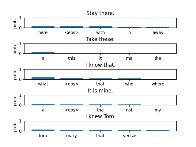
Unlike the previous example, Python code: Bigram-count-based.py displays the top five most probable words for each prediction. . This provides a broader view of the model’s output.
$ python Bigram-count-based.py
=================================
Using Bigram
vocabulary size: 302
number of sentences: 7452
=================================
Text:Stay there.
Predicted last word:
	here	=> 0.185185
	<eos>	=> 0.129630
	with	=> 0.111111
	in	=> 0.101852
	away	=> 0.092593

Text:Take these.
Predicted last word:
	a	=> 0.157895
	this	=> 0.078947
	it	=> 0.065789
	me	=> 0.065789
	the	=> 0.065789

Text:I know that.
Predicted last word:
	what	=> 0.191489
	<eos>	=> 0.096927
	that	=> 0.078014
	who	=> 0.073286
	where	=> 0.061466

Text:It is mine.
Predicted last word:
	a	=> 0.082759
	<eos>	=> 0.068966
	the	=> 0.067816
	not	=> 0.065517
	my	=> 0.035632

Text:I knew Tom.
Predicted last word:
	tom	=> 0.138298
	mary	=> 0.085106
	that	=> 0.085106
	<eos>	=> 0.063830
	it	=> 0.063830
As expected, the results suggest that the model’s accuracy is not high.
11.1.2. Trigram Model
A trigram model approximates the conditional probability of the language model as follows:
$$ P(w_{i}|w_{\lt i}) \thickapprox P(w_{i}| w_{i-2}, w_{i-1}) \tag{11.8} $$Using $(11.8)$, a trigram language model is expressed as follows:
$$ P(w_{1:n}) = P(w_{1}) P(w_{2}|w_{1}) P(w_{3}|w_{1}, w_{2}) \cdots P(w_{n}|w_{n-2},w_{n-1}) = P(w_{2}|w_{1}) \prod_{i=3}^{n} P(w_{i}| w_{i-2}, w_{i-1}) $$since $P(w_{1}) = P(\lt \negthinspace \negthinspace \text{SOS} \negthinspace \negthinspace \gt) = 1$.
11.1.2.1. Last Word Prediction Task
The last word prediction is defined as follows:
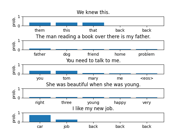
$$ \hat{w}_{n} = \underset{w \in V}{argmax} \ P(w| w_{n-2}, w_{n-1}) $$Python code: Trigram-count-based.py displays the top five most probable words for each prediction.
$ python Trigram-count-based.py
=================================
Using Trigram
vocabulary size: 302
number of sentences: 7452
=================================
Text:We knew this.
Predicted last word:
	them	=> 0.333333
	this	=> 0.333333
	that	=> 0.333333

Text:The man reading a book over there is my father.
Predicted last word:
	father	=> 0.129032
	dog	=> 0.064516
	friend	=> 0.064516
	home	=> 0.064516
	problem	=> 0.064516

Text:You need to talk to me.
Predicted last word:
	you	=> 0.316456
	tom	=> 0.316456
	mary	=> 0.075949
	me	=> 0.063291
	<eos>	=> 0.050633

Text:She was beautiful when she was young.
Predicted last word:
	right	=> 0.093750
	three	=> 0.093750
	young	=> 0.093750
	happy	=> 0.062500
	very	=> 0.062500

Text:I like my new job.
Predicted last word:
	car	=> 0.750000
	job	=> 0.250000
Even though the model achieves slightly better accuracy than the bigram model, its overall performance remains low.
Surprisingly, n-gram models with improvements like smoothing remained dominant in NLP until the early 2010s.
The most astonishing thing while studying NLP for this document was that the concept of Markov chains was introduced by Markov in 1913, in the context of early NLP research, rather than in the field of mathematics.
Speech and Language Processing (3rd Edition draft) (Chapter 3, “Bibliographical and Historical Notes”) mentions the following explanation:
The underlying mathematics of the n-gram was first proposed by Markov (1913), who used what are now called Markov chains (bigrams and trigrams) to predict whether an upcoming letter in Pushkin’s Eugene Onegin would be a vowel or a consonant. Markov classified 20,000 letters as V or C and computed the bigram and trigram probability that a given letter would be a vowel given the previous one or two letters.