7.5. Back Propagation Through Time in Many-to-Many type
The formulation of the Many-to-Many simple RNN with dense layers is defined as follows:
$$ \begin{cases} \hat{h}^{(t)} = W x^{(t)} + U h^{(t-1)} + b \\ h^{(t)} = f(\hat{h}^{(t)}) \\ \hat{y}^{(t)} = V h^{(t)} + c \\ y^{(t)} = g(\hat{y}^{(t)}) \end{cases} \tag{7.10} $$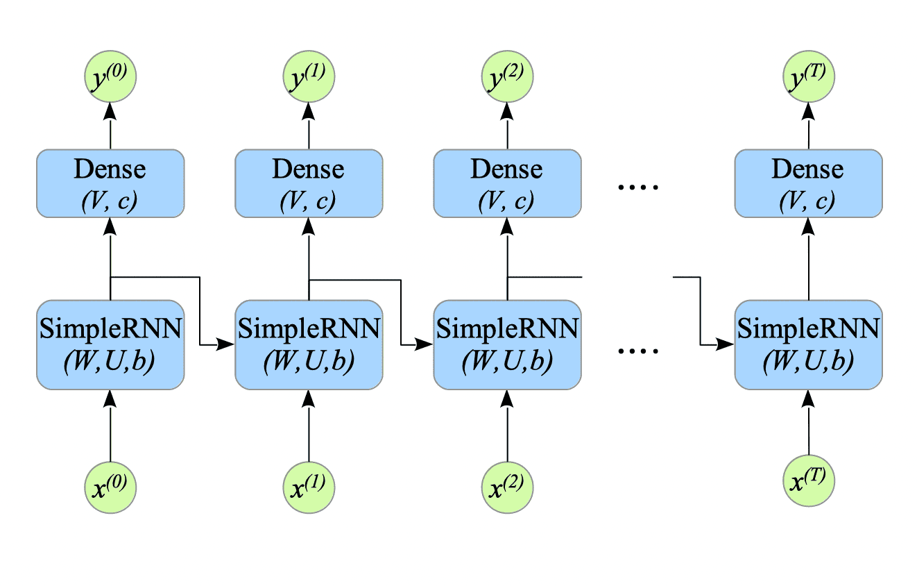
Fig.7-8: Many-to-Many SimpleRNN
7.5.1. Computing the gradients for Back Propagation Through Time
We use the mean squared error (MSE) as the loss function $L$, defined as follows:
$$ L = \sum_{t=0}^{T} \frac{1}{2} (y^{(t)} - Y^{(t)})^{2} \tag{7.11} $$For convenience, we define $L^{(t)}$, the loss value at time step $t$:
$$ L^{(t)} \stackrel{\mathrm{def}}{=} \frac{1}{2} (y^{(t)} - Y^{(t)})^{2} \tag{7.12} $$Thus, the loss function $L$ can be represented as follows:
$$ L = \sum_{t=0}^{T} L^{(t)} \tag{7.13} $$To simplify the following discussion, we define the following expression:
$$ \text{grad}_{dense}^{(t)} \stackrel{\mathrm{def}}{=} \frac{\partial L^{(t)}}{\partial h^{(t)}} \tag{7.14} $$$ \text{grad}_{dense}^{(t)}$ is the gradient propagated from the dense layer at time step $t$.
Using these expressions, we can build the backward computational graph shown in Fig.7-9.
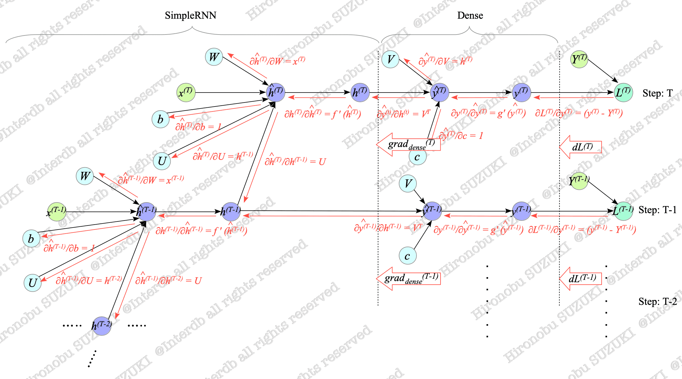
Fig.7-9: Backward Computational Graph of Many-to-Many SimpleRNN
For an explanation of computational graphs, see Appendix.
Fig.7-10 illustrates the relationship between $h^{(T)}$ and $h^{(T-1)}$, which is extracted from Fig.7-9.
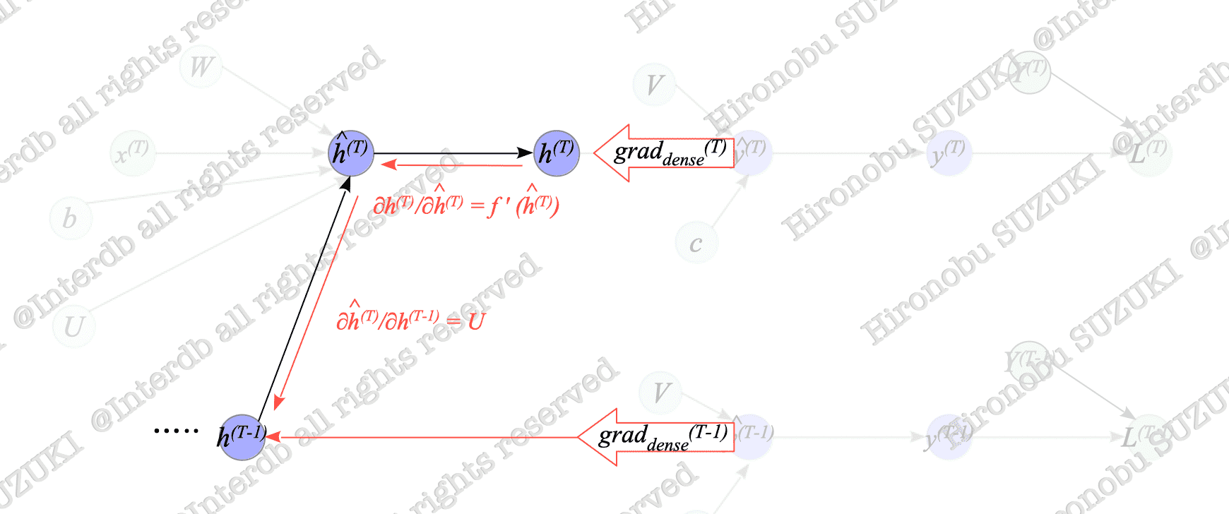
Fig.7-10: Relationship Between $h^{(T)}$, $h^{(T-1)}$, and Dense Layer Outputs
As shown in Fig.7-10, The difference between the many-to-many type and many-to-one type of $h^{(T-1)}$ is whether or not $\text{grad}_{dense}^{(T-1)}$ is added.
We can derive $dh^{(t)}$ for a many-to-many RNN from expression $(7.6)$ as follows:
$$ dh^{(t)} = \begin{cases} \text{grad}_{dense}^{(t)} & t = T \\ \\ \text{grad}_{dense}^{(t)} + dh^{(t+1)} f'(\hat{h}^{(t+1)}) \ {}^t U & 0 \le t \lt T \end{cases} \tag{7.15} $$To avoid confusion, we express the transpose of a vector or matrix $ A $ as $ {}^tA$, instead of $A^{T}$, in this section.
Finally, we can compute the gradients $dW$, $dU$, and $db$, defined in expressions $(7.7)-(7.9)$ in Section 7.2.4, using the $dh^{(t)}$ defined in $(7.15)$.