11.3. Language Modeling with RNN

In Part 2, we demonstrated RNNs’ ability to predict the next value in a numerical sequence. Now, let’s explore how they can be used for a more complex task: predicting the next word in a sentence.
We can represent an RNN as follows:
$$ h_{t} = \begin{cases} 0 & t = 0 \\ r(w_{t}, h_{t-1}) & t \gt 0 \end{cases} \tag{11.9} $$where:
- $r(\cdot)$ is any recurrent neural network such as simple RNN, LSTM or GRU.
- $h_{t}$ is the hidden state of the recurrent neural network $r(\cdot)$ at time step $t$.
- $w_{t}$ is an input word at time step $t$.
To predict the next word $w_{t+1}$ given a sequence ${w_{1}, w_{2},\ldots, w_{t}}$, we use a dense layer with a softmax activation function as follows:
$$ P(w_{t+1}|w_{1}, w_{2},\ldots, w_{t}) = \text{softmax}(W h_{t}) \tag{11.10} $$where:
- $W \in \mathbb{R}^{|V| \times d_{h}}$ is a weight matrix belonging to a dense layer with no bias.
- $V$ is a set of vocabulary.
- $d_{h}$ is the hidden state dimension.
Using $(11.10)$, we can naturally define a language model such as $(11.5)$, and also the last word prediction task using RNN can be defined as follows:
$$ \hat{w}_{n} = \underset{w \in V}{argmax} \ P(w| w_{\lt n}) = \underset{w \in V}{argmax} \ \text{softmax}(W h_{n-1}) \tag{11.11} $$In the following subsections, we will create an RNN-based language model and employ it to perform last-word prediction.
11.3.1. Implementation
Complete Python code is available at: LanguageModel-RNN-tf.py
11.3.1.1. Create Model
To build our RNN-based language model, we employ a many-to-many GRU neural network shown below:
# ========================================
# Create Model
# ========================================

input_nodes = 1
hidden_nodes = 1024
output_nodes = vocab_size

embedding_dim = 256

class GRU(tf.keras.Model):
    def __init__(self, hidden_units, output_units, vocab_size, embedding_dim):
        super().__init__()
        self.hidden_units = hidden_units
        self.embedding = tf.keras.layers.Embedding(vocab_size, embedding_dim)
        self.gru = tf.keras.layers.GRU(
            self.hidden_units,
            return_sequences=True,
            return_state=False,
            recurrent_initializer="glorot_uniform",
        )
        self.softmax = tf.keras.layers.Dense(output_units, activation="softmax")

    def call(self, x):
        x = self.embedding(x)
        output = self.gru(x)
        x = self.softmax(output)
        return x


model = GRU(hidden_nodes, output_nodes, vocab_size, embedding_dim)

model.build(input_shape=(None, max_len))
This code is similar to the sine wave prediction model in Section 9.4.1, with three key differences:
-
Many-to-Many GRU Layer: As mentioned above, this model has a Many-to-Many architecture. Therefore, we set $\text{return_sequences}=\text{True}$ to return the entire sequence of hidden states $\text{output}$.
-
Dense Layer: The activation function of the dense layer is the softmax function. Its output size equals the size of the dictionary (vocabulary), providing probabilities for each word in the vocabulary.
-
Word Embedding Layer: The input (tokenized data) is passed through the word embedding layer before being fed into the GRU unit. Hence, the GRU unit internally handles the vector data corresponding to the input.
11.3.1.2. Dataset and Training
An RNN-based language model predicts the next word in a sequence based on the previous words in the sentence.
Let $x_{1}, x_{2}, \ldots , x_{n}$ represents an input word sequence. The corresponding desired output sequence $y$ is constructed by shifting the input sequence by one word and appending a special padding symbol “<pad>” at the end:
$$ y_{1}, y_{2}, \ldots , y_{n} = x_{2}, x_{3}, \ldots, x_{n}, \lt \!\! \text{pad} \!\! \gt $$Example:
INPUT : <SOS> just   go    for    it     <EOS>
OUTPUT: just  go     for   it     <EOS>  <pad>
In this example, the RNN-based language model would be trained to:
- predict ‘just’ from <SOS>.
- predict ‘go’ from ‘just’.
- predict ‘for’ from ‘go’.
- predict ‘it’ from ‘for’.
- predict <EOS> from ‘it’.
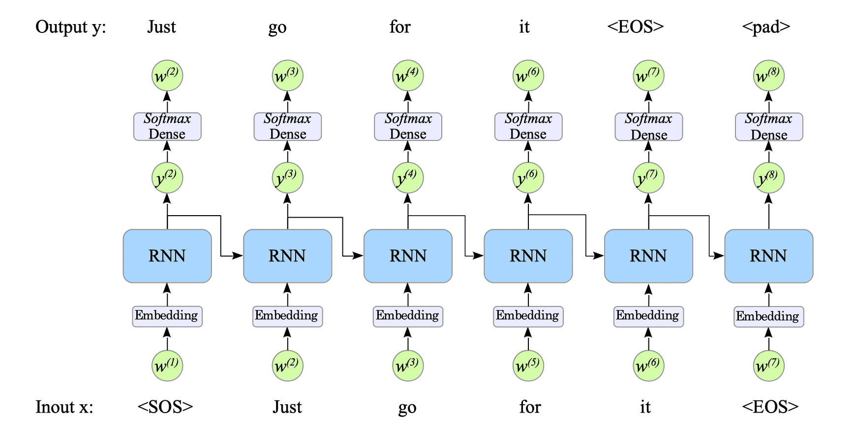
Fig.11-2: Training Process in Our Language Model
The training phase is almost identical to the one described in the previous parts, involving RNNs and XOR gates.
# ========================================
# Training
# ========================================

lr = 0.0001
beta1 = 0.99
beta2 = 0.9999

optimizer = optimizers.Adam(learning_rate=lr, beta_1=beta1, beta_2=beta2)


@tf.function
def train(x, y):
    with tf.GradientTape() as tape:
        output = model(x)
        loss = loss_function(y, output)
        grad = tape.gradient(loss, model.trainable_variables)
    optimizer.apply_gradients(zip(grad, model.trainable_variables))
    return loss


# If n_epochs = 0, this model uses the trained parameters saved in the last checkpoint,
# allowing you to perform last word prediction without retraining.
if len(sys.argv) == 2:
    n_epochs = int(sys.argv[1])
else:
    n_epochs = 200

for epoch in range(1, n_epochs + 1):

    for batch, (X_train, Y_train) in enumerate(dataset):
        loss = train(X_train, Y_train)
We use the SparseCategoricalCrossentropy as the loss function because our training data $y$ is a set of integers, like “$[21 \ \ 1 \ \ 44 \ \ 0 \ \ 0]$”.
If you are concerned about the difference between the output format of the GRU (softmax output) and the training data format, refer to the documentation.
loss_object = tf.keras.losses.SparseCategoricalCrossentropy(reduction="none")

def loss_function(real, pred):
    mask = tf.math.logical_not(tf.math.equal(real, 0))  # this masks '<pad>'
    """
    Example:

    real= tf.Tensor(
    [[21  1 44 0  0]   (jump !    <eos> <pad> <pad>)
    [ 17  9 24 2 44]   (i    go   there .     <eos>)
    [ 27  1 44 0  0]   (no   !    <eos> <pad> <pad>)
    [ 21 22 32 2 44]], (i    know you   .     <eos>)
    , shape=(4, 5), dtype=int64)

    where <pad> = 0.

    mask= tf.Tensor(
    [[True  True  True False False]
    [ True  True  True True  True ]
    [[True  True  True False False]
    [ True  True  True True  True ],
    shape=(4, 5), dtype=bool)
    """

    loss_ = loss_object(real, pred)
    mask = tf.cast(mask, dtype=loss_.dtype)
    loss_ *= mask
return tf.reduce_mean(loss_)This loss function is also used in the machine translation models, in Sections 13.2.3 of seq2seq-tf.py and 14.4.2 of seq2seq-tf-attention.py.
11.3.1.3. Prediction
For the last word prediction task, we feed our language model with the input sequence excluding the last word.
The resulting output sequences from the model are then passed to the softmax layer. The output of the softmax layer represents the probabilities of each word in the vocabulary.
We select the most probable word as the predicted last word by picking the last element of the output of the softmax layer.
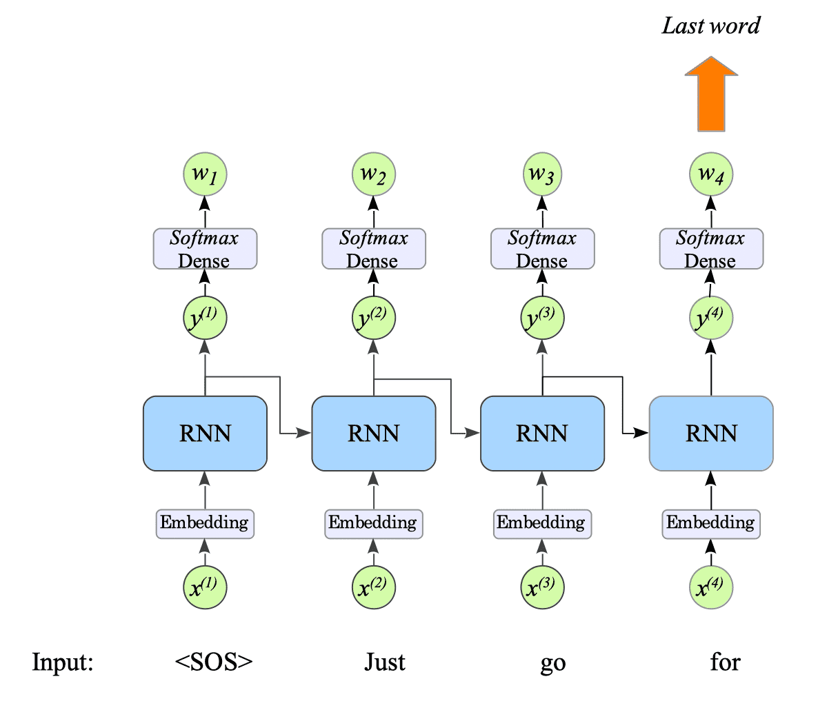
Fig.11-3: Prediction Process in Our Language Model
11.3.2. Demonstration
Following 200 epochs of training, our RNN-based language model’s last-word prediction is shown below:
$ python LanguageModel-RNN-tf.py
=================================
vocabulary size: 303
number of sentences: 7452
=================================
Model: "gru"
_________________________________________________________________
 Layer (type)                Output Shape              Param #
=================================================================
 embedding (Embedding)       multiple                  77568

 gru_1 (GRU)                 multiple                  3938304

 dense (Dense)               multiple                  310575

=================================================================
Total params: 4,326,447

... snip ...

Text:  Just let me help you.
Input: <sos> Just let me help
Predicted last word:
	you	=> 0.857351
	the	=> 0.005812
	i	=> 0.002887
	me	=> 0.002504
	tom	=> 0.002407

Text:  Tom is the one who told me who to give it to.
Input: <sos> Tom is the one who told me who to give it
Predicted last word:
	to	=> 0.924526
	time	=> 0.001423
	this	=> 0.000225
	if	=> 0.000026
	your	=> 0.000024

Text:  She will get well soon.
Input: <sos> She will get well
Predicted last word:
	soon	=> 0.855645
	in	=> 0.032168
	very	=> 0.011623
	here	=> 0.008390
	old	=> 0.007782

Text:  I came back home late.
Input: <sos> I came back home
Predicted last word:
	late	=> 0.836478
	alone	=> 0.032124
	by	=> 0.031414
	with	=> 0.027323
	night	=> 0.002223

Text:  She told me that I could use her room.
Input: <sos> She told me that i could use her
Predicted last word:
	room	=> 0.930203
	with	=> 0.011007
	car	=> 0.010192
	brother	=> 0.003243
	father	=> 0.002974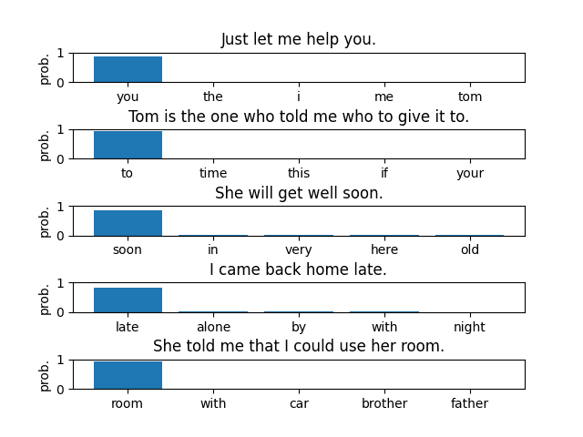
This code contains the checkpoint function that preserves the training progress. Hence, once trained, the task can be executed without retraining by setting the parameter $\text{n_epochs}$ to $0$, or simply passing $0$ when executing the Python code, as shown below:
$ python LanguageModel-RNN-tf.py 0