13.1. Training and Translation
In the encoder-decoder model, the encoder’s core function remains the same in both training and translation phases. It involves extracting information from the source language and passing the final state to the decoder as a context vector.
In contrast, the decoder’s behavior changes depending on the phase (training or translation).
- Training: The decoder learns to predict the next words of the target language sequence using the context vector as its initial value.
- Translation: It relies on its own previously generated outputs to predict the next word, building the complete sentence one step at a time.
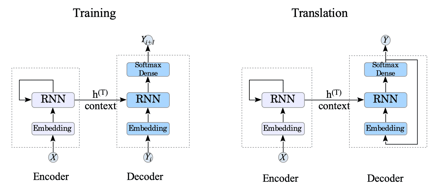
Fig.13-2: (Left) Training Phase. (Right) Translation Phase.
Focusing on the training phase, the encoder-decoder model is simpler to understand its architecture. It can be viewed as a combination of two familiar models: a sentence classification model and a language model.
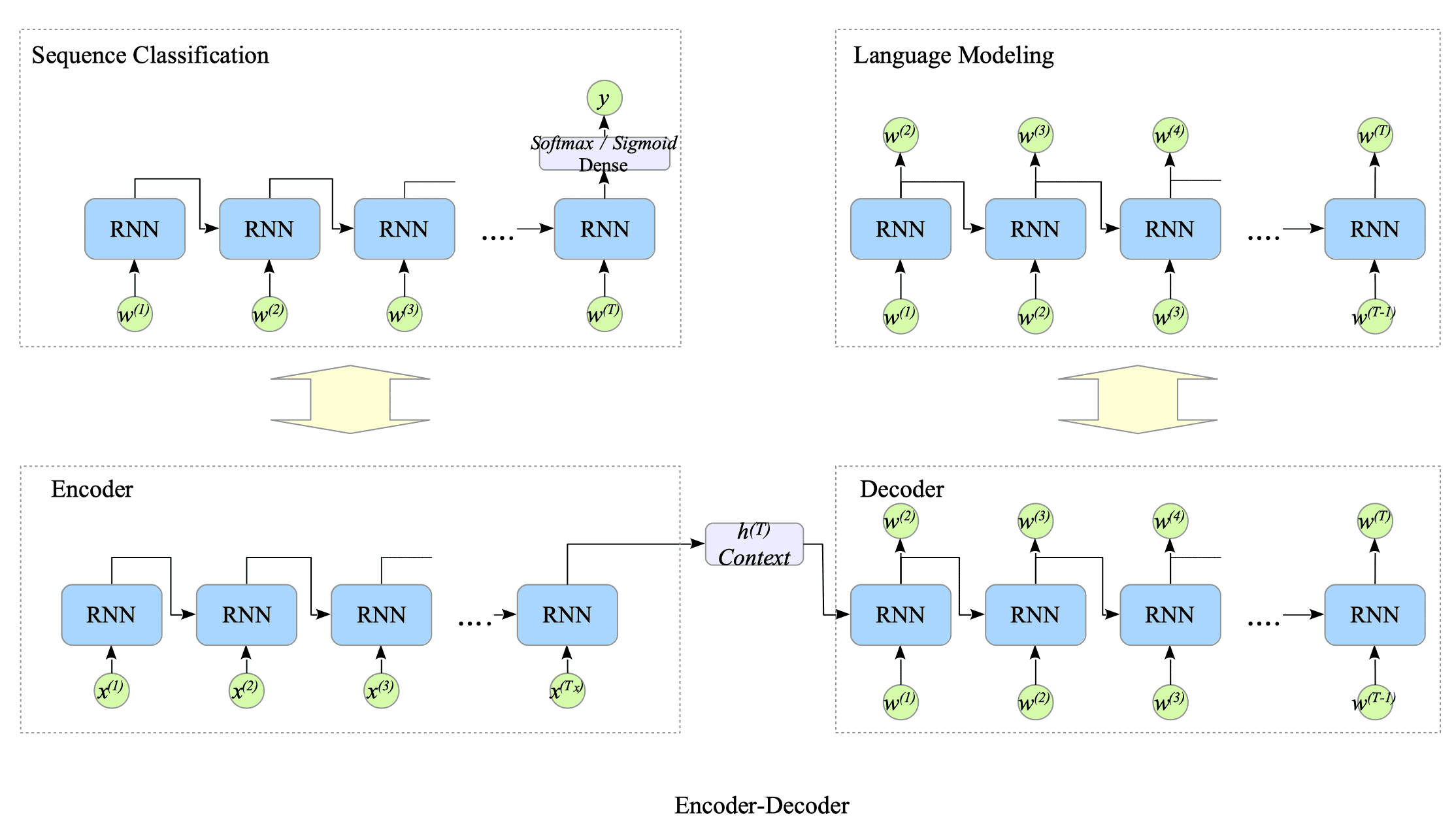
Fig.13-3: Relationship Between the Three Model Architectures During Training
Fundamentally, the decoder constructs a language model that simply predicts the next word in the input sequence for the target language through training.
In the following, we will delve into the encoder-decoder model in both training and translation phases.
13.1.1. Training
Let’s explore how this model trains using the following dataset.
- Source sentence: “<SOS> Yo soy Hironobu . <EOS>”
- Target sentence: “<SOS> I am Hironobu . <EOS>”.
When the model receives the above dataset, the encoder and the decoder performs as follows:
-
Encoder: The encoder processes the source sentence “<SOS> Yo soy Hironobu . <EOS>”, and then passes the context vector, which captures the essence of the sentence, to the decoder.
-
Decoder: Using the context vector as an initial value, the decoder is trained to predict the next word in the target language $Y_{i+1}$ based on the previous word $Y_{i}$. This process starts with the “<SOS>” token as the initial input and continues until before the “<EOS>” token.
In this example, the decoder is trained to predict the sequence “I am Hironobu . <EOS>” from “<SOS> I am Hironobu .”.
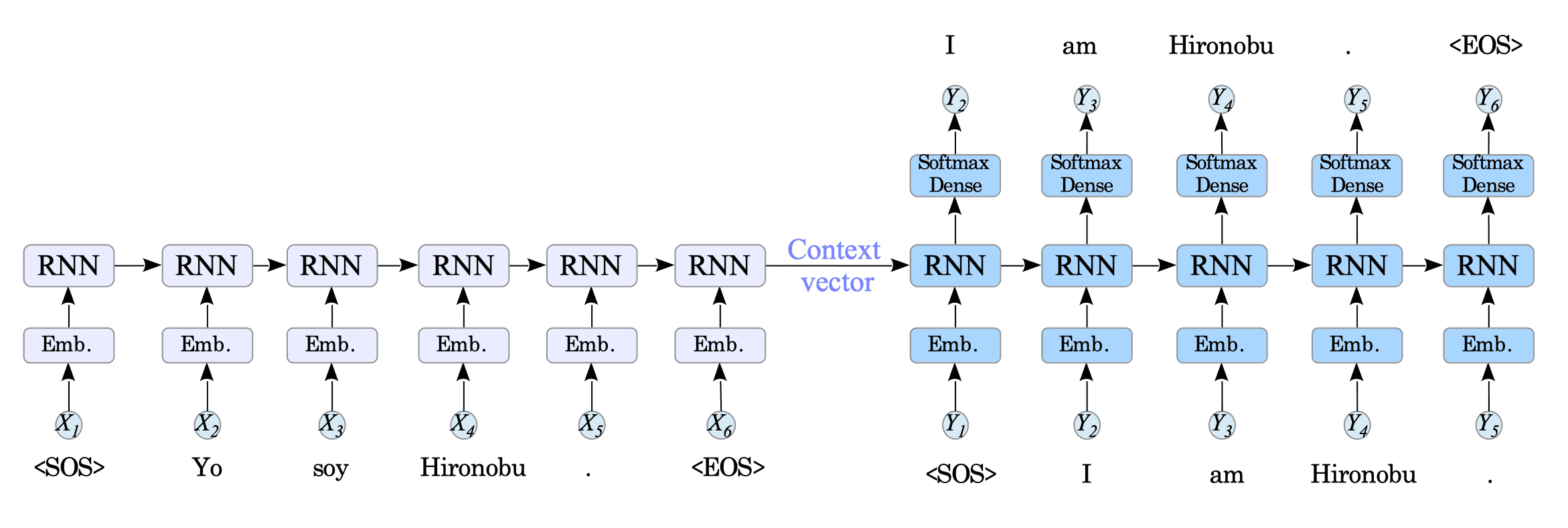
Fig.13-4: Encoder-Decoder Model in Training
In training phase, the decoder’s gradient $dh_{d}^{(0)}$ is propagated back to the encoder, and it is used to adjust the weights and bias of the encoder.
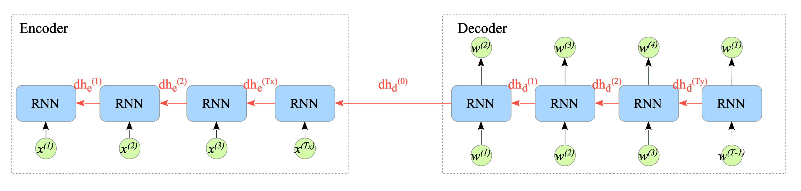
Fig.13-5: Pseudo-Backward Computational Graph of RNN-Based Encoder-Decoder Model
This means that the decoder’s errors are propagated back to the encoder, which not only improves the decoder’s performance but also enhances the encoder’s ability to capture the context of source sentences.
13.1.2. Translation
In the translation phase, the decoder takes the context vector from the encoder, and generates the target language sequence.
The decoder is already trained to generate the next token from the previous token in the target language. One thing to consider is which token to choose from the output of the decoder. Due to the softmax activation function, the decoder predicts probabilities for all tokens in its vocabulary at each step.
Here are three methods for approaching this task: greedy search, exhaustive search, and beam search.
13.1.2.1. Greedy Search
The simplest approach to generate the translated sentence is to choose the word with the highest probability at each step. This approach is called greedy search.
For example, if we represent the start-of-sentence token <SOS> as $y_{1}$ and the context vector as $c$, the next token $y_{2}$ can be obtained as follows:
$$ y_{2} = \underset{y \in V}{argmax} \ P(y| c, y_{1}) $$Similarly, it continues step-by-step, predicting the subsequent token, $y_{i}$, based on the previous token, $y_{i-1}$, until it reaches the end-of-sentence <EOS> token.
$$ y_{i} = \underset{y \in V}{argmax} \ P(y| c, y_{\lt i}) $$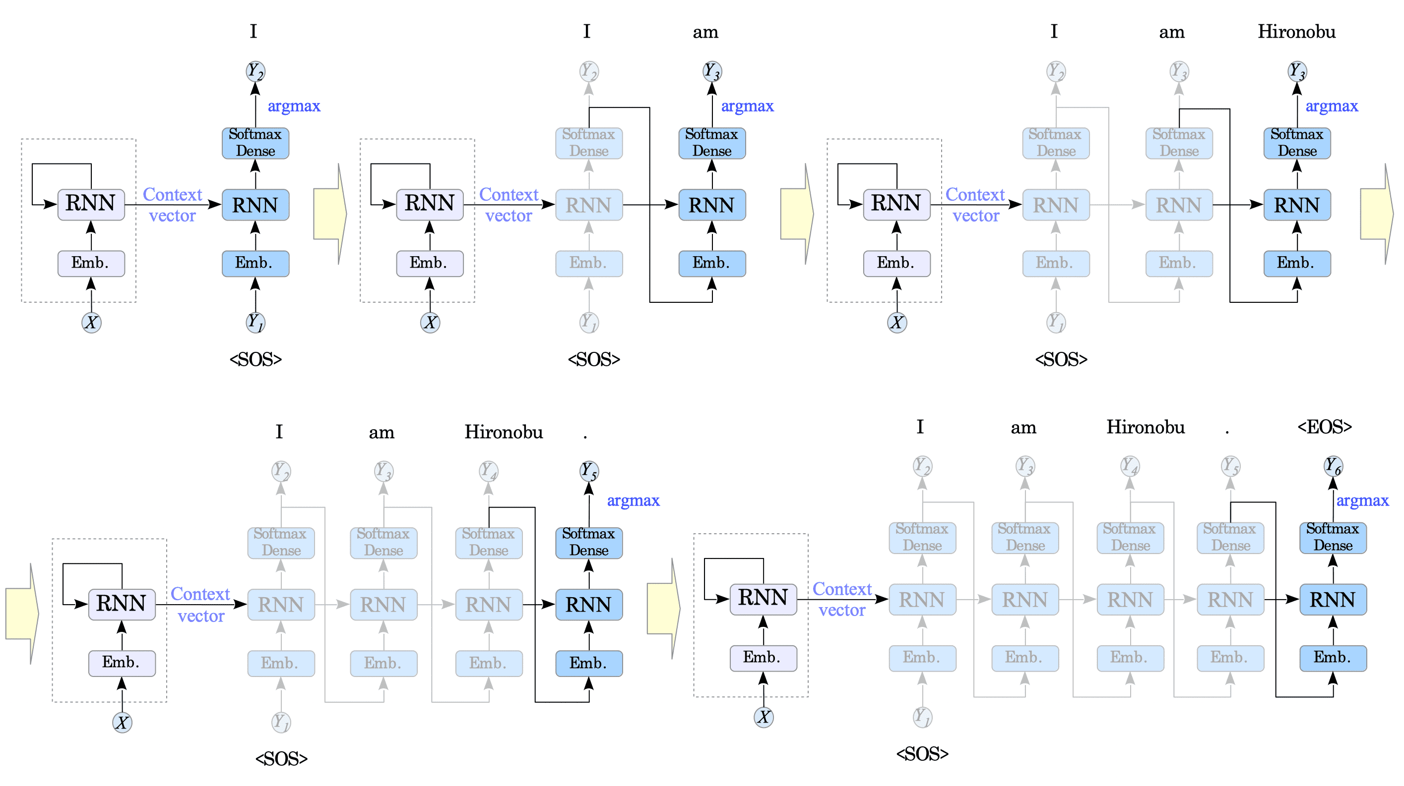
Fig.13-6: Encoder-Decoder Model in Translation with Greedy Search
Greedy search seems intuitive, but it can be risky, like walking a tightrope.
If the decoder makes a mistake at an early step (e.g., predicting $y_{2}$ incorrectly), it is likely to keep making errors throughout the sequence. This is called error propagation.
Despite this disadvantage, we will use greedy search in this document because of its simplicity and relative effectiveness.
13.1.2.2. Exhaustive Search
Exhaustive search considers all possible combinations of tokens in the vocabulary. While it would be the best approach to translate sentences, it is computationally impractical.
Consider a sentence translation task with a vocabulary of $10,000$ words. A $10$-word sentence has $10,000^{10} = 10^{40}$ possible translations, while a $20$-word sentence has $10^{80}$ possibilities. These are astronomical numbers1.
13.1.2.3. Beam Search
Beam search offers a middle ground between greedy search and exhaustive search. It considers a limited set of the most promising candidate translations, expanding them at each step. This approach is more efficient than exhaustive search while overcoming the limitations of greedy search.
Beam search maintains a set of the most promising translations, called the beam. At each step, the beam is expanded by generating all possible continuations of the current beam candidates. These continuations are then scored using a language model, and the top-scoring ones are added to the beam, replacing lower-scoring candidates. The beam search algorithm terminates when it reaches a goal (the end-of-sentence token <EOS>) or after a certain number of steps.
-
The age of the universe is only $ 1.36 \times 10^{10}$[years] $= 4.29 \times 10^{17}$ [sec]. The size of the observable universe is $8.8 \times 10^{26}$ [m]. The weight of the observable universe is $1.5 \times 10^{53}$ [kg]. The number of protons in the observable universe is $10^{80}$. ↩︎