7.2. Computing the gradients for Back Propagation Through Time
Implementing the backpropagation procedure for a simple RNN requires calculating parameter gradients. The steps are similar to those used in ordinary neural networks:
- Define the loss function.
- Construct the forward computational graph to build the backward graph.
- Build the backward computational graph by calculating derivatives between nodes of the forward graph, considering sequence information.
- Obtain all parameter gradients Utilizing the backward computational graph.
Following these steps, we will calculate the gradients for all parameters in the Simple RNN.
7.2.1. Loss function
Since our task is a regression problem, we will use the mean squared error (MSE) as our loss function. The MSE is defined as follows:
$$ L = \frac{1}{2} (y^{(T)} - Y^{(T)})^{2} \tag{7.3} $$7.2.2. Forward Computational Graph
Fig.7-5 illustrates the forward computational graph of the simple RNN.
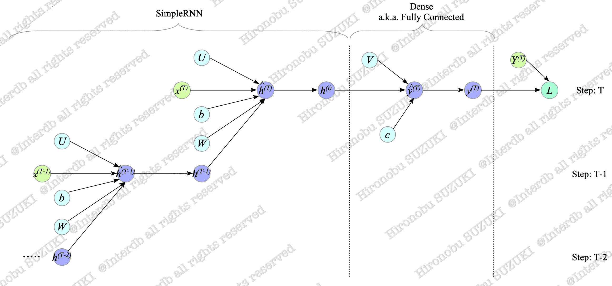
Fig.7-5: Forward Computational Graph of Many-to-One SimpleRNN
For an explanation of computational graphs, see Appendix.
7.2.3. Backward Computational Graph
To build the backward computational graph, we will calculate the derivatives between nodes of the above graph.
Since the derivatives of the dense layer have been calculated in Section 4.1, we focus on calculating the derivatives of the SimpleRNN.
$$ \begin{align} \frac{\partial h^{(t)}}{\partial \hat{h}^{(t)}} &= \frac{\partial f(\hat{h}^{(t)})}{\partial \hat{h}^{(t)}} = f'(\hat{h}^{(t)}) \\ \frac{\partial \hat{h}^{(t)}}{\partial U} &= \frac{\partial (W x^{(t)} + U h^{(t-1)} + b)}{\partial U} = {}^t h^{(t-1)} \\ \frac{\partial \hat{h}^{(t)}}{\partial W} &= \frac{\partial (W x^{(t)} + U h^{(t-1)} + b)}{\partial W} = {}^t x^{(t)} \\ \frac{\partial \hat{h}^{(t)}}{\partial b} &= \frac{\partial (W x^{(t)} + U h^{(t-1)} + b)}{\partial b} = 1 \\ \frac{\partial \hat{h}^{(t)}}{\partial h^{(t-1)}} &= \frac{\partial (W x^{(t)} + U h^{(t-1)} + b)}{\partial h^{(t-1)}} = {}^t U \end{align} $$To avoid confusion, we express the transpose of a vector or matrix $ A $ as $ {}^t A$, instead of $A^{T}$, in this section.
Using these derivatives we calculated, we can build the backward computational graph shown in Fig.7-6.
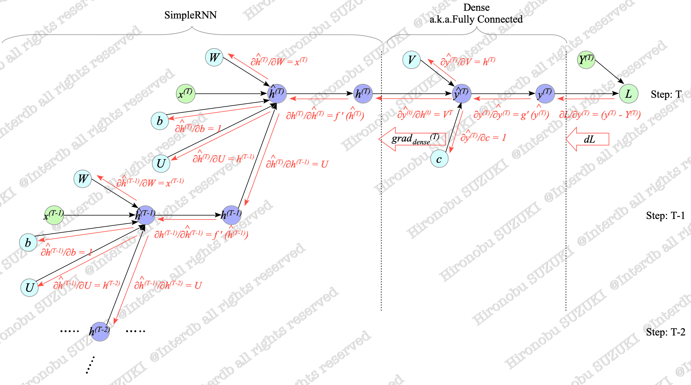
Fig.7-6: Backward Computational Graph of Many-to-One SimpleRNN
Fig.7-6 illustrates a simplified backward computational graph at time steps $T$ and $T-1$, but gradients actually back-propagate through all time steps up to $0$.
Therefore, to obtain the final gradients, we must calculate them at each time step and then add them together. This process is known as backpropagation through time (BPTT).
7.2.3.1. BackPropagation Through Time (BPTT)
Gradients flow through the current hidden state $h^{(t)}$ to the previous state $h^{(t-1)}$. This allows us to recursively calculate gradients for all time steps based on this relationship.
To simplify the discussion, we define the following expressions:
$$ \begin{align} \text{grad}_{dense}^{(T)} & \stackrel{\mathrm{def}}{=} \frac{\partial L}{\partial h^{(T)}} \tag{7.4} \\ dh^{(t)} & \stackrel{\mathrm{def}}{=} \frac{\partial L}{\partial h^{(t)}} \tag{7.5} \end{align} $$- $\text{grad}_{dense}^{(T)}$ is the gradient propagated from the dense layer.
- $dh^{(t)}$ is the gradient propagated from the hidden state $h^{(t+1)}$.
In this document, “$d$” denotes the gradient (e.g., $dL, dh$), not the total derivative.
By definition, $dh^{(T)} = \text{grad}_{dense}^{(T)}$.
Next, we will calculate $dh^{(T-1)}$. Fig.7-7 illustrates the relationship between $h^{(T)}$ and $h^{(T-1)}$, which is extracted from Fig.7-6.
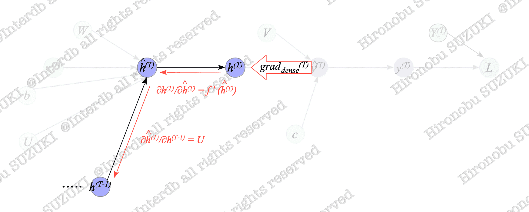
Fig.7-7: Relationship Between $h^{(T)}$ and $h^{(T-1)}$
As shown in Fig.7-7, $ dh^{(T-1)} $ can be calculated from $ dh^{(T)} $:
$$ \begin{align} dh^{(T-1)} &= \frac{\partial L}{\partial h^{(T-1)}} = \frac{\partial L}{\partial h^{(T)}} \frac{\partial h^{(T)}}{\partial \hat{h}^{(T)}} \frac{\partial \hat{h}^{(T)}}{\partial h^{(T-1)}} = dh^{(T)} f'(\hat{h}^{(T)}) \ {}^t U \end{align} $$Similarly, $ dh^{(t)} $ can be also calculated recursively:
$$ dh^{(t)} = \begin{cases} \text{grad}_{dense}^{(t)} & t = T \\ \\ dh^{(t+1)} f'(\hat{h}^{(t+1)}) \ {}^t U & 0 \le t \lt T \end{cases} \tag{7.6} $$7.2.4. Gradients
Using the results above, we finally obtain the gradients as shown below:
$$ \begin{align} dW &\stackrel{\mathrm{def}}{=} \frac{\partial L}{\partial W} = \sum_{t=0}^{T} \frac{\partial L}{\partial h^{(t)}} \frac{\partial h^{(t)}}{\partial \hat{h}^{(t)}} \frac{\partial \hat{h}^{(t)}} {\partial W} = \sum_{t=0}^{T} dh^{(t)} f'(\hat{h}^{(t)}) \ {}^t x^{(t)} \tag{7.7} \\ dU &\stackrel{\mathrm{def}}{=} \frac{\partial L}{\partial U} = \sum_{t=1}^{T} \frac{\partial L}{\partial h^{(t)}} \frac{\partial h^{(t)}}{\partial \hat{h}^{(t)}} \frac{\partial \hat{h}^{(t)}} {\partial U} = \sum_{t=1}^{T} dh^{(t)} f'(\hat{h}^{(t)}) \ {}^t h^{(t-1)} \tag{7.8} \\ db &\stackrel{\mathrm{def}}{=} \frac{\partial L}{\partial b} = \sum_{t=0}^{T} \frac{\partial L}{\partial h^{(t)}} \frac{\partial h^{(t)}}{\partial \hat{h}^{(t)}} \frac{\partial \hat{h}^{(t)}} {\partial b} = \sum_{t=0}^{T} dh^{(t)} f'(\hat{h}^{(t)}) \tag{7.9} \end{align} $$