2.2. Differential Calculus
This section will introduce key concepts from differential calculus, which are also essential building blocks for understanding deep learning.
2.2.1. Essential Derivatives Cheat Sheet
- $ \log(x) $
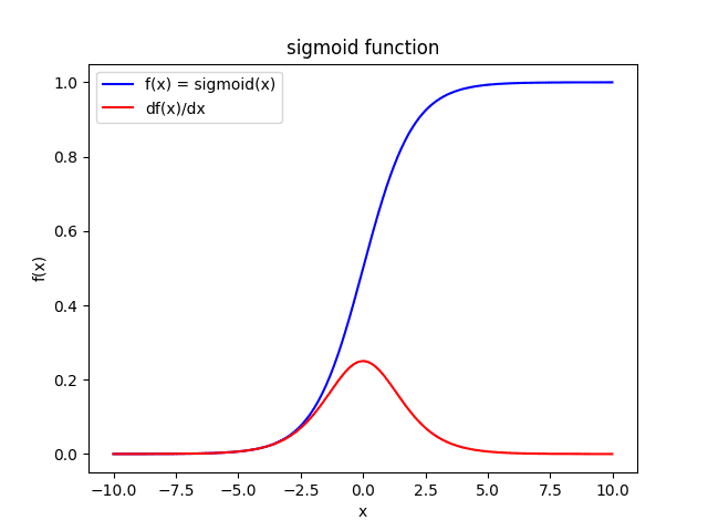
- $ sigmoid(x) = \sigma(x) = \frac{1}{1 + \exp(-x)} $
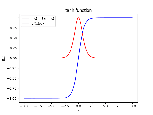
- $ tanh(x) $
- $f(x) = g(x)h(x) $
- $f(x) = g(x)/h(x) $
2.2.2. Chain Rule
In differential calculus, the chain rule helps us differentiate composite functions.
Imagine a function $f(\cdot)$ that depends on another function $g(x)$, resulting in $f(g(x))$. The chain rule allows us to find the derivative of $f(g(x))$ with respect to $x$. This is expressed as:
$$ \frac{d f(g(x))}{d x} = \frac{d f(g(x))}{d g(x)} \frac{d g(x)}{d x} $$- Example 1: $ y = \sin(2x+3)$
- Example 2:
2.2.3. Computational Graph
A computational graph is a directed graph that represents a mathematical expression. The nodes in the graph represent operations or variables, and the edges represent the dependencies between them.
For example, the equation $ y = \sin(ax+b)$ can be represented as a computational graph in Fig.2-1:
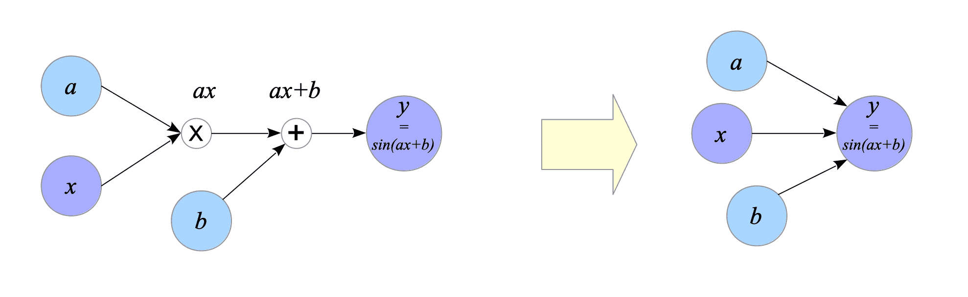
Fig.2-1: (Left) Computational Graph of $y = \sin(ax+b)$. (Right) Simplified Computational Graph of the Left Graph.
As shown in the above figure, the operation nodes can be removed to simplify the graph.
One more example is shown in Fig.2-2:
$$ \begin{cases} y = \sin(ax+b) \\ z = y^{2} \end{cases} $$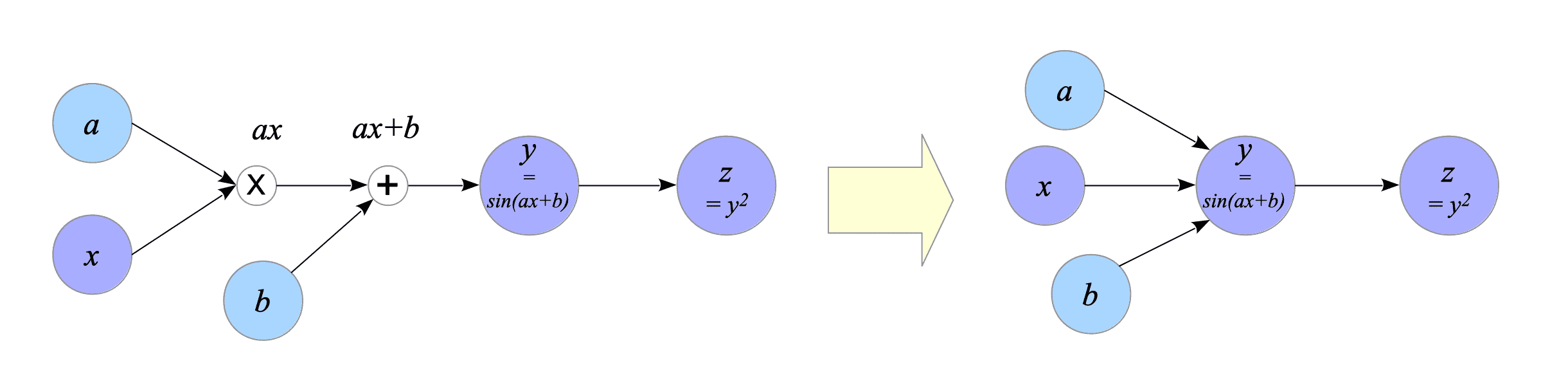
Fig.2-2: (Left) Computational Graph of {$y=\sin(ax+b)$; $z=y^{2}$}. (Right) Simplified computational Graph of the Left Graph.
Computational graphs can be classified into two types:
- Forward computational graph: This type represents the order of operations in a mathematical expression. The graph above is an example of a forward computational graph.
- Backward computational graph: This type represents the order of operations in calculating the derivatives of a mathematical expression.
In deep learning, backward computational graphs are crucial because they help us compute the derivatives of complex functions. As explained in Part 1, almost half of deep learning’s computations involve computing derivatives.
When using deep learning frameworks such as TensorFlow, we do not need to do differential computation explicitly, but when learning deep learning theory, backward computational graphs help us understand it.
Creating a backward computational graph is relatively simple:
- Draw a differentiation symbol ($\frac{d}{d}$) between each node.
- Place the left node variable in the numerator and the right node variable in the denominator.
- Perform the differentiation.
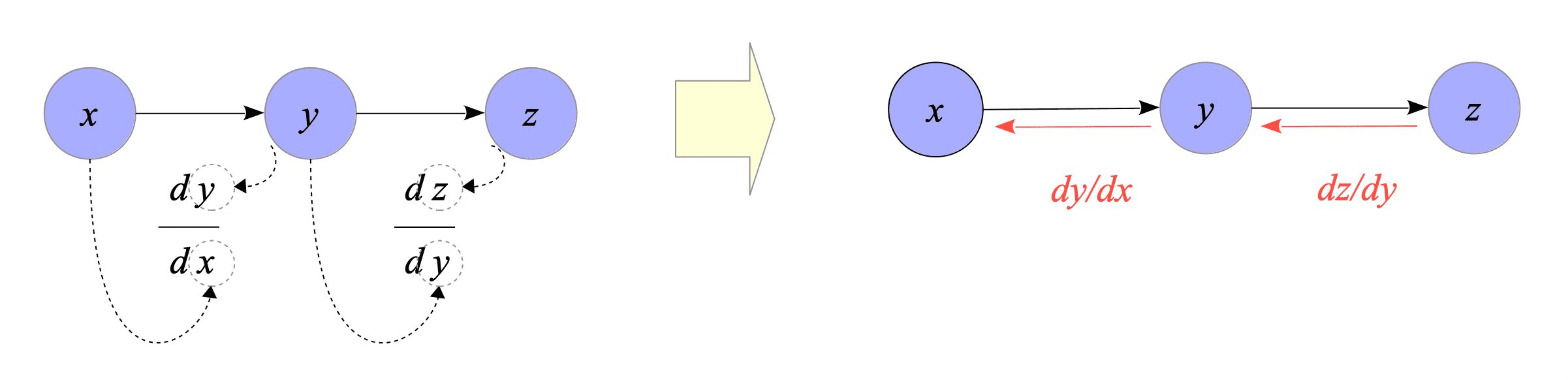
Fig.2-3: Creating a Backward Computational Graph
As you can see from the above graph, it can be said that backward computational graphs are visualizations of the chain rule.
Example:
Let’s calculate the derivative $\frac{dz}{dx}$ of the following equations:
$$ \begin{cases} y = 2x^{3}+3 \\ z = y^{2} \end{cases} $$First, we create the backward computational graph, i.e., calculate $\frac{dz}{dy}$ and $\frac{dy}{dx}$.
$$ \begin{align} \frac{d z}{d y} &= \frac{d y^{2}}{d y} = 2y \\ \frac{d y}{d x} &= \frac{d (2x^{3} + 3)}{d x} = 6x^{2} \end{align} $$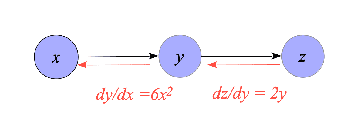
Fig.2-4: Backward Computational Graph of {$y=2x^{3}+3$; $z=y^{2}$}.
Next, we calculate $\frac{dz}{dx}$ by multiplying the derivatives from right to left on the backward computational graph.
$$ \frac{d z}{d x} = \frac{d z}{d y} \frac{d y}{d x} = 2y \cdot 6x^{2} = 12 x^{2}(2x^{3}+3) $$2.2.4. Automatic differentiation
In Part 1 or later, it will become clear that almost half of the computations in deep learning are spent on computing derivatives.
According to the article “Automatic Differentiation in Machine Learning: a Survey”, methods for the computation of derivatives in computer programs are divided into four categories:
- Manually coded
- Numerical differentiation (e.g., Newton’s method)
- Symbolic differentiation (e.g., Mathematica, Maxima, and Maple)
- Automatic differentiation (e.g., autograd, Jax, and AutoDiff)
Modern deep learning frameworks have adopted the fourth approach, i.e., using automatic differentiation systems. For instance, TensorFlow uses AutoDiff, and PyTorch uses its own automatic differentiation system.
Example:
Let’s calculate $\frac{dz}{dx}$ of the following equations:
$$ \begin{cases} y = 2x^{3}+3 \\ z = y^{2} \end{cases} $$The following code shows the values of $\frac{dz}{dx}$ when $x =0.5$, calculated by using the result of the previous subsection and by using autograd.
>>> from autograd import grad
>>>
>>> x = 0.5
>>>
>>> #
>>> # Calculate manually
>>> #
>>> _grad = 12 * x**2 * (2*x**3 + 3)
>>> _grad
9.75
>>>
>>> #
>>> # Compute automatically using autograd
>>> #
>>>
>>> def z(x):
...     y = 2 * x**3 + 3
...     z = y**2
...     return z
...
>>> gradient_fun = grad(z)
>>> _grad = gradient_fun(x)
>>> _grad
9.75