21.1. Model Formulation
Alpha Version: Work in progress.
This section presents the model formulation and loss function for GPT-1 fine-tuning, using Natural Language Inference (NLI) as an example.
21.1.1. Model Formulation
NLI tasks involve predicting the relationship label between a pair of input sentences. Consequently, its architecture builds directly upon the Sequence Classification model introduced in Chapter 12.
The fine-tuning architecture takes the final transformer output representation $h_{L}$ and passes it through a linear (dense) layer followed by a softmax function to generate class predictions.
During fine-tuning, the premise and hypothesis are concatenated into a single input sequence $X$ and fed into the pre-trained GPT-1 model. The hidden representation corresponding to the final token, denoted as $h_{L}^{m}$, is projected via a linear layer (with weight matrix $W_{y}$) and transformed by softmax to compute the class probability distribution.
Figure 21.2 illustrates the overall fine-tuning architecture.
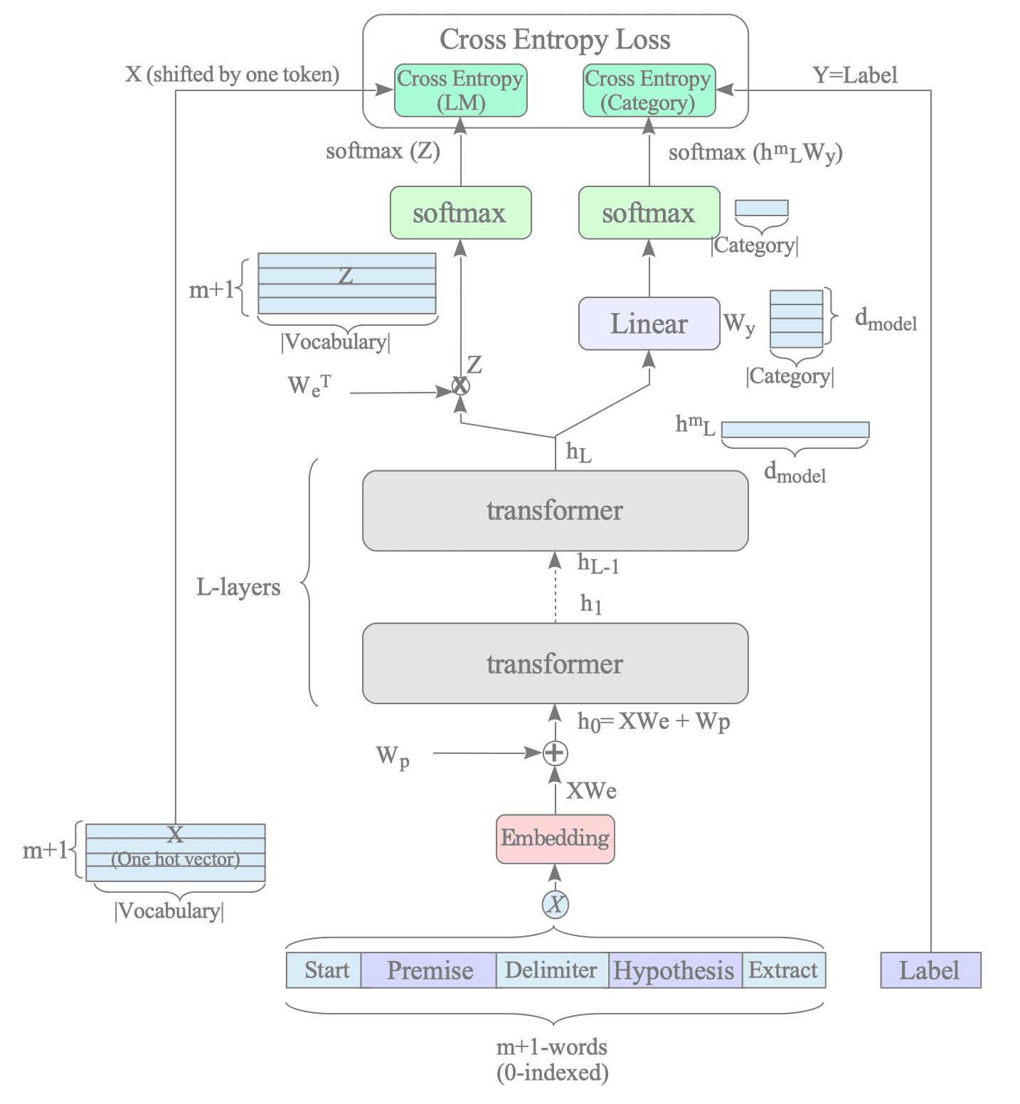
Fig.21-2: GPT-1 Fine-Tuning Model.
Let the input sequence $X$ be represented as
$$ X = [x^{0}, \ldots, x^{m}], $$
and the target class label $y$ as
$$y \in \lbrace 0, \ldots, \vert{}\text{Category}\vert{}-1 \rbrace.$$
Let $h_{L}^{m}$ denote the hidden representation of the final input token (i.e., the last row of $h_{L}$). The predicted output probability vector $P \in \mathbb{R}^{\vert{}\text{Category}\vert{}}$ is computed as follows:
$$ P = \operatorname{softmax}(h_{L}^{m}W_{y}) $$
where:
- $P \in \mathbb{R}^{\vert{}\text{Category}\vert{}}$ is the predicted class probability vector.
- $h_{L}^{m} \in \mathbb{R}^{1 \times d_{\text{model}}}$ is the hidden representation of the final input token.
- $W_{y} \in \mathbb{R}^{d_{\text{model}} \times \vert{}\text{Category}\vert{}}$ is the weight matrix of the linear classification layer.
21.1.2. Loss Function
With the classifier defined, the model is trained by minimizing the categorical cross-entropy loss $L_{c}$.
The categorical cross-entropy loss $L_{c}$ is formulated as:
$$L_{c} = - \sum_{k=1}^{\vert{}\text{Category}\vert{}} Y_{k} \log(P(y_{k}\mid x^{0}, \ldots, x^{m}))$$
where:
- $Y \in \mathbb{R}^{\vert{}\text{Category}\vert{}}$ is the one-hot encoded ground-truth vector for label $y$.
- $Y_k \in \lbrace 0,1 \rbrace$ denotes the $k$-th element of $Y$, where $Y_k = 1$ for the target class and $Y_k = 0$ otherwise.
If the true class index is $c$, the one-hot vector $Y$ can be expressed as:
$$ Y = \underbrace{ [0,\ldots,0,\overset{c\text{-th}}{1},0,\ldots,0] }_{|\text{Category}|} $$Consequently, the classification loss $L_{c}$ simplifies to:
$$L_{c} = - \log(P(y_{c}\mid x^{0}, \ldots, x^{m}))$$
However, optimizing solely for the task-specific classification loss risks degrading the general language modeling capabilities acquired during pre-training—a phenomenon known as catastrophic forgetting.
To mitigate this issue, GPT-1 fine-tuning incorporates the auxiliary language-model loss $L_{p}$ alongside the categorical cross-entropy loss $L_{c}$.
Specifically, the overall fine-tuning objective function $L_{f}$ is defined as a weighted sum of both losses:
$$L_{f} = L_{c} + \lambda L_{p}$$
where $\lambda \in [0,1]$ is a hyperparameter balancing the two loss components. The original GPT-1 implementation adopts $\lambda = 0.5$.
The auxiliary loss $L_{p}$ is computed over the same input sequence by predicting the next token at each position, following the exact procedure outlined in Chapter 20.
Including this auxiliary objective helps retain pre-trained language knowledge while adapting the model to downstream target tasks.
21.1.3. Implementation
The following function computes the categorical cross-entropy loss $L_{c}$:
def clf_loss_fn(labels, logits):
    """
    Classification cross-entropy

    Parameters
    ----------
    labels : (B,)    integer class indices  {0=entailment, 1=neutral, 2=contradiction}
    logits : (B, 3)  raw classification logits

    Returns
    -------
    Scalar mean cross-entropy over the batch.
    """
    loss = tf.keras.losses.sparse_categorical_crossentropy(
        labels, logits, from_logits=True
    )  # (B,)
    return tf.reduce_mean(loss)
The function below constructs the fine-tuning step, computing the joint loss $L_{f}$:
def make_finetune_step(model: GPT1ForNLI, optimizer, lm_coef: float, grad_clip: float):
    """
    Return a @tf.function-compiled fine-tuning step for *model*.

    The returned function implements the joint objective from Eq. 5:
        Lf = Lc(clf) + \lambda \dot Lp(lm)

    It updates:
        train_loss     <- Lf (joint)
        train_clf_loss <- Lc (classification only)
        train_lm_loss  <- Lp (auxiliary LM only)
        train_accuracy <- NLI classification accuracy
    """

    @tf.function(input_signature=_finetune_step_signature)
    def finetune_step(input_ids, labels):
        """
        One gradient-update step on a (premise, hypothesis, label) batch.

        input_ids : (B, T)  NLI-format sequences  <s> premise $ hypothesis </s>
        labels    : (B,)    integer class  {0=entailment, 1=neutral, 2=contradiction}

        Forward (GPT-1 Section 3.2 & 3.3):
          clf_logits  = Wy \dot h_n^{</s>}                   -> Lc (classification)
          lm_logits   = softmax(h_n \dot We^T)  at all steps  -> Lp (auxiliary LM)
          Lf = Lc + \lambda \dot Lp
        """
        with tf.device(DEVICE):
            with tf.GradientTape() as tape:
                clf_logits, lm_logits, _ = model(input_ids, training=True)
                # clf_logits : (B, 3)
                # lm_logits  : (B, T, V)

                # Lc: NLI classification loss
                c_loss = clf_loss_fn(labels, clf_logits)

                # Lp: auxiliary LM loss on the NLI sequence
                # Position j predicts token j+1 within the full sequence.
                lm_targets = input_ids[:, 1:]  # (B, T-1)  next tokens
                lm_pred = lm_logits[:, :-1, :]  # (B, T-1, V)  shifted logits
                l_loss = lm_loss_fn(lm_targets, lm_pred)

                # Lf: joint objective (Eq. 5)
                total = c_loss + lm_coef * l_loss

            gradients = tape.gradient(total, model.trainable_variables)
            gradients, _ = tf.clip_by_global_norm(gradients, grad_clip)
            optimizer.apply_gradients(zip(gradients, model.trainable_variables))

        train_loss(total)
        train_clf_loss(c_loss)
        train_lm_loss(l_loss)
        train_accuracy.update_state(labels, clf_logits)

    return finetune_step